Short Communication

A New European Slope Length and Steepness Factor (LS-Factor) for Modeling Soil Erosion by Water

by
Panos Panagos
1,*,
Pasquale Borrelli
1,† and
Katrin Meusburger
2,†
1
European Commission, Joint Research Centre, Institute for Environment and Sustainability, Via Enrico Fermi 2749, I-21027 Ispra (VA), Italy
2
Environmental Geosciences, University of Basel, Bernoullistrasse 30, 4056 Basel, Switzerland
*
Author to whom correspondence should be addressed.
These authors contributed equally to this work.
Geosciences 2015, 5(2), 117-126; https://doi.org/10.3390/geosciences5020117
Submission received: 24 December 2014 / Revised: 23 March 2015 / Accepted: 23 March 2015 / Published: 3 April 2015

Abstract

:
The Universal Soil Loss Equation (USLE) model is the most frequently used model for soil erosion risk estimation. Among the six input layers, the combined slope length and slope angle (LS-factor) has the greatest influence on soil loss at the European scale. The S-factor measures the effect of slope steepness, and the L-factor defines the impact of slope length. The combined LS-factor describes the effect of topography on soil erosion. The European Soil Data Centre (ESDAC) developed a new pan-European high-resolution soil erosion assessment to achieve a better understanding of the spatial and temporal patterns of soil erosion in Europe. The LS-calculation was performed using the original equation proposed by Desmet and Govers (1996) and implemented using the System for Automated Geoscientific Analyses (SAGA), which incorporates a multiple flow algorithm and contributes to a precise estimation of flow accumulation. The LS-factor dataset was calculated using a high-resolution (25 m) Digital Elevation Model (DEM) for the whole European Union, resulting in an improved delineation of areas at risk of soil erosion as compared to lower-resolution datasets. This combined approach of using GIS software tools with high-resolution DEMs has been successfully applied in regional assessments in the past, and is now being applied for first time at the European scale.

Graphical Abstract

1. Introduction

Soil erosion is a land degradation process that impacts a number of functions (biodiversity, food production, carbon stock, ecosystem services), the precise quantitate assessment of which can be modeled. The Universal Soil Loss Equation (USLE) and its revised version (RUSLE) are frequently used in soil erosion modeling even at large scales, despite their shortcomings. In a data collection exercise performed at the European level in 2009–2010 through a network of national contact points, almost all soil erosion modelers who provided data at national level used the RUSLE model [1]. The main input layers for the USLE model are rainfall erosivity (R-factor), soil erodibility (K-factor), vegetation cover (C-factor), slope length and slope angle (LS-factor) and the support practice (P-factor). As the LS- and C-factors have the greatest impact on modeling soil loss [2], it is important to continue to improve the accuracy of these factors.
The Digital Elevation Model (DEM) is a quantitative representation of the Earth’s surface that provides basic information about the terrain and allows for the derivation of attributes such as slope, aspect, drainage area and network, curvature, and topographic index [3]. The DEM and the LS factor determine the spatial resolution (cell size) of the soil erosion model results, and incorporate the soil erosion potential due to surface runoff. The L-factor gives the impact of slope length while the S-factor accounts for the effect of slope steepness. The LS-factor is dimensionless, having values equal to and greater than 0. The main objective of this study is to compute the LS-factor based on a high-resolution DEM for the whole European Union. Most European-scale studies [4,5] implemented the LS-factor using the algorithms proposed by Desmet and Govers (1996) [6].

2. Methodology

The methodology presented in this paper for estimating the LS-factor has the following features: (a) uses a high-resolution DEM at 25 m, (b) applies the Desmet and Govers (1996) algorithm [6], and (c) limits the estimation of LS to a maximum slope angle of 50% (26.6 degrees).
We used a new high-resolution (25 m) DEM of the European Union (EU-DEM) to calculate the LS-factor. The EU-DEM provides pan-European elevation data at 1 arc-second, and is a hybrid product based mainly on Shuttle Radar Topography Mission (SRTM) and Advanced Spaceborne Thermal Emission and Reflection Radiometer (ASTER) Global Digital Elevation Model (GDEM) [7]. The EU-DEM was developed through the Copernicus program, and its statistical validation documents a relatively satisfactory overall vertical accuracy of 2.9 m root mean square error [8]. This resolution of the EU-DEM is the best available at the European scale; to date, only regional [9,10] or national soil erosion estimates have used DEMs with resolutions of 10 to 40 m [1]. Molnar and Julien (1998) [11] calculated soil erosion at different grid-cell resolutions. They concluded that the grid-cell size is very important for the S-factor, since the slope decreases as the cell size increases.
Initially, McCool et al. (1987) [12] found that soil loss occurs faster in slopes that were steeper than 9%. Renard et al. (1997) [13] adopted this algorithm in RUSLE for the S-factor estimation based on the slope gradient:
S = 10.8 × sin Θ + 0.03, where slope gradient < 0.09
S = 16.8 × sin Θ − 0.5, where slope gradient ≥ 0.09
where Θ is the gradient of slope in degrees.
Compared to other methodologies applied in China [14], which use a different algorithm for steeper slopes (>10 degrees), the S-factor calculated using this method is lower by around 20%. This difference between our methodology and Liu’s algorithm could be attributed to the fact that 45% of the areas studied in the EU-DEM contained slopes that were greater than 10 degrees. This difference is minimal in agricultural land uses as very limited arable areas are found in steep slopes. However, the RUSLE algorithm [13] was selected in order to be able to compare results with those of other studies carried out in the European Union.
Initially, Wischmeier and Smith (1978) [15] defined the L-factor as the ratio of soil lost from a horizontal slope length to the corresponding loss from the slope length of a unit plot (22.13 m). According to this definition, slope length is the distance from the point of origin of overland flow to the point where either the slope gradient decreases enough for deposition to start, or runoff waters are streamed into a channel. According to this simple definition, the L-factor can be represented as:
L = ( λ 22.13 ) m
where λ is the slope length (in meters) and m is equivalent to 0.5 for slopes steeper than 5%, 0.4 for slopes between 3%–4%, 0.3 for slopes between 1%–3% and 0.2 for slopes less than 1%.
Given that slope steepness is not uniform for the whole area, Foster and Wischmeier (1974) [16] proposed to sub-divide the slope into a number of segments. Desmet and Govers (1996) [6] extended this approach to a two-dimensional terrain using the concept of the unit-contributing area:
L i , j = ( A i , j i n +   D 2 ) m + 1   A i , j i n m + 1   D m + 2   *   x i , j m   *   22.13 m
where A i , j i n   is the contributing area at the inlet of grid cell (i,j) measured in m2. D is the grid cell size (meters), Xi,j = sin a i , j + cos a i , j , the a i , j is the aspect direction of the grid cell (i,j).
m is related to the ratio β of the rill to interill erosion:
m = β β + 1
where,
β = sin θ 0.0896 [ 0.56   +   3 * ( sin θ ) 0.8 ]
θ is the slope angle in degrees. The m ranges between 0 and 1, and approaches 0 when the ratio of rill to interill erosion is close to 0 [17]. Contrary to Mitasova et al. (1996) [18], Desmet and Govers (1997) [19] proved that this LS-factor model is appropriate for landscape-scale soil erosion modeling, and can capture complex topography.
The cutoff slope angle is defined as the change in slope angle from one cell to the next. The maximum slope angle for which the LS-factor is estimated is 50%. This option was selected both using the values suggested in the literature [20], [21] and by performing experimental estimations in Switzerland, which has the highest slope gradients and the most heterogeneous geomorphology in Europe. Both McCool et al. (1993) [22] in the United States and Liu et al. (2000) [23] in China defined the maximum slope angle as 55% for LS-factor estimation. Hardly any type of soil above 50% slope angle was found in Europe. Only 1.3% of the forests and 0.5% of grasslands are on slopes in Switzerland that are steeper than 26.6 degrees (50%). Having tested this hypothesis in Switzerland, it was obvious that very few (0.003%) cells in the European Union territory could have a slope greater than 50%. Therefore, the cutoff value of 50% was assigned.
The increasing availability of DEMs has promoted the use of image-processing techniques and software for deriving terrain properties [24] such as the LS-factor. SAGA (System for Automated Geoscientific Analyses) software is a user-friendly platform that provides a comprehensive set of modules for data analysis and numerous applications such as those focusing on DEMs and Terrain Analysis [25,26]. We estimated the LS-factor by using one of the hydrology modules available in SAGA (the LS-factor field base) which incorporates the multiple flow algorithm [27]. Moreover, SAGA carries out computations much more quickly than the classical ArcGIS toolbox [28], and calculates flow accumulation directly from the DEMs.
The main limitation of this methodology is the existence of landscape features (i.e., roads, paths, fences, contours, stone walls and grass margins) that may interrupt the water runoff and reduce the slope length, but are not identified in the DEM. The 25 m DEM could be potentially used for the identification of such features, but would involve an unsustainable amount of processing time and effort at the European scale. Experimental results on the island of Crete [29] have demonstrated that local landscape features result in a proportional reduction of the LS-factor. Those characteristics may be useful for calibrating LS-factor estimations at national or European scales. However, features which are maintained by farmers, such as grass margins, contours and stone walls, are proposed among the support practices (P-factor) that help reduce soil erosion.

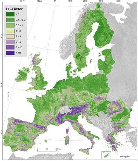
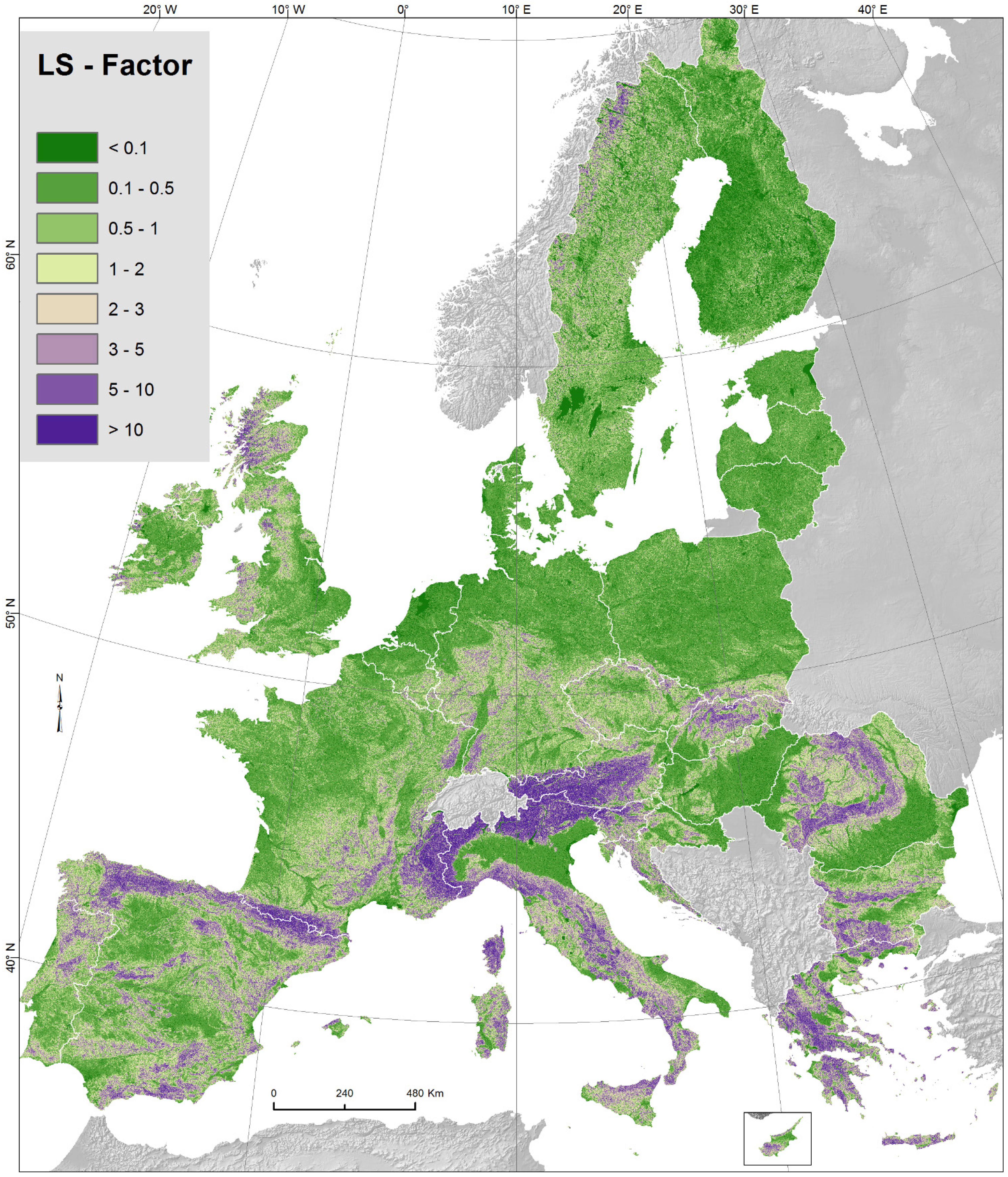
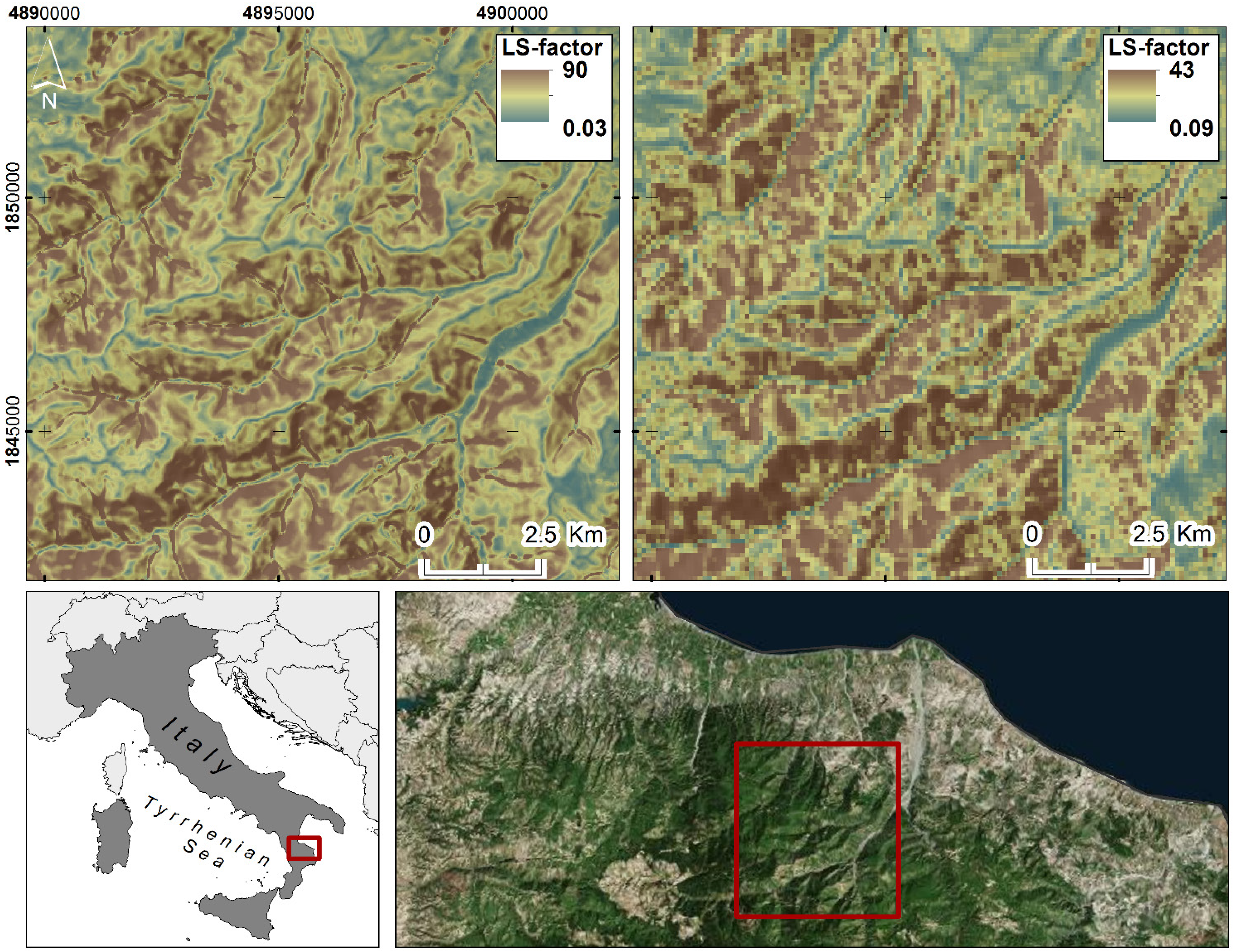
3. Results and Discussion

The application of the methodology resulted in the first topographic mapping of the LS-factor at 25-m resolution for the European Union (Figure 1). The greatest LS-factor values are observed in mountain areas such as the Alps (Slovenia, Austria, Italy and France), the Pyrenees (Spain), the Apennines (Italy), the Carpathian mountains (Romania) and the Pindos mountain range (Greece). The mean LS-factor value for the whole European Union is 1.63, with a range of 0 to 99. LS-factor values greater than 25 were found in only 0.1% of the whole European Union, mainly located in Austria, Greece, Italy and Slovenia.
The calculation of some descriptive statistics (mean, standard deviation, coefficient of variation) helped identify the countries with the highest mean LS-factor values due to their complex topography, characterized mainly by undulating relief. Austria has the highest mean LS-factor (5.2) followed by Slovenia, Greece, and Italy, each with mean LS-factors greater than 3 (Table 1). The flattest country is the Netherlands (LS-factor = 0.2) followed by Denmark, the Baltic States and Finland (LS < 0.5).
The Coefficient of variation (CV) is an indicator of the degree of heterogeneity within a country. The greatest variation is found in France, Hungary and Poland, while the least variation is found in the Baltic States, Luxembourg and the Netherlands. Moreover, the aggregated data allow for a quick estimation of the influence of the LS-factor in the overall soil loss rates of a country. More detailed statistics per land cover type can be found in Table S1.
Figure 1. Slope length and steepness factor (LS-factor) in the European Union.
Geosciences 05 00117 g001
Table 1. LS-factor statistics per country. More detailed statistics per land cover type can be found in Table S1.
Country NameCodeMeanStandard DeviationCoefficient of Variation
AustriaAT5.205.911.14
BelgiumBE0.680.951.40
BulgariaBG2.343.001.28
CyprusCY2.312.721.18
Czech Rep.CZ1.361.571.15
GermanyDE1.051.641.57
DenmarkDK0.320.341.07
EstoniaEE0.320.310.96
SpainES2.242.971.33
FinlandFI0.410.641.56
FranceFR1.723.121.81
GreeceGR3.794.051.07
CroatiaHR1.892.561.36
HungaryHU0.590.991.69
IrelandIE1.011.541.52
ItalyIT3.634.861.34
LithuaniaLT0.350.381.09
LuxembourgLU1.621.681.04
LatviaLV0.390.360.93
MaltaMT1.341.971.46
NetherlandsNL0.190.201.05
PolandPL0.520.861.67
PortugalPT1.802.251.25
RomaniaRO2.092.821.35
SwedenSE0.991.511.52
SloveniaSI3.874.211.09
SlovakiaSK2.572.841.11
United KingdomUK1.402.021.45
In a recent pan-European study, Bosco et al. (2015) [30] have estimated the LS-factor based on 100 m DEM (much coarser resolution than the current one) using a simplified equation and assuming surface runoff concentration in less than 300 m. Instead, our approach has taken as input the high resolution DEM at 25 m, employed a multiple flow algorithm for the flow accumulation and did not apply any arbitrary slope lengths. The detailed features that are shown in the 25 m DEM are obscured in the coarser resolution (100 m) with loss of drainage network patterns and hillslopes variability. The spatial variability of landscape features and the LS-factor increased accuracy of our study are visible (Figure 2) compared to past study [30]. As DEM resolution and accuracy increase, the landscape will be more accurately described, soil erosion topographic factor will be calculated precisely and erosion estimates will approach actual values [31]. Wu et al. (2005) [32] concluded that the 30 m DEM resolution is adequate for soil erosion assessments while the 100 m should be handled with care due to increased contributing area and decreased slopes.
Due to its high (25 m) resolution, the European LS-factor dataset is more than 50GB in size. LS-factor datasets per country can be downloaded from the European Soil Data Centre (ESDAC) web platform [33] and used as input layers for any soil erosion assessment at various scales (local, regional, national, European). The use of GIS software tools (e.g., SAGA) with the high-resolution DEM allows for precise soil erosion estimates with more reasonable costs and better accuracy than in the past. The LS-factor, combined with the K-factor at 500-m resolution [34], the R-factor at 500-m resolution [35], the P-factor [36] and the upcoming C-factor layer, will greatly help to improve soil erosion modeling at the European scale.
Figure 2. Comparison of LS-factor in the current study (upper left) with Bosco et al. (2015) [30] (upper right) in Calabria area (Southern Italy).
Geosciences 05 00117 g002

4. Conclusions

The LS-factor has been calculated in great detail using the high-resolution 25 m DEM, the multiple flow algorithm and the SAGA software. The visual analysis (Figure 2) indicates that DEM resolution does have profound consequence on the spatial pattern of the LS factor. This first application of a DEM at this scale for the whole European Union is a significant improvement on past assessments that used 100 m DEMs due to higher input data accuracy, multiple flow algorithm implementation and better representation of landscape. The high-resolution DEM helps to capture the geomorphological changes with greater precision and thereby estimate soil erosion with greater accuracy compared to past assessments. The latest software developments such as SAGA have contributed significantly to this improvement. As DEM resolution increases, the landscape is more accurately modeled contributing to better spatial soil loss estimates.
The quality of the modeled LS-factor is considered to be sufficient for the European scale as it mainly uses the high-resolution (25 m) DEM. The availability of real data is also important for soil erosion modelers, particularly when applying the complex LS-factor algorithms.

Acknowledgments

The authors would like to thank Gráinne Mulhern for the revision of the article from a linguistic point of view.

Author Contributions

Panos Panagos and Pasquale Borrelli conceived and designed the experiments; Pasquale Borrelli and Katrin Meusburger performed the experiments; Panos Panagos and Pasquale Borrelli analyzed the data; Pasquale Borrelli, Katrin Meusburger, Panos Panagos contributed reagents/materials/analysis tools; Panos Panagos and Pasquale Borrelli wrote the paper.

Supplementary Materials

Supplementary materials can be accessed at: https://www.mdpi.com/2076-3263/5/2/117/s1.

Conflicts of Interest

The authors declare no conflict of interest.

References

  1. Panagos, P.; Meusburger, K.; van Liedekerke, M.; Alewell, C.; Hiederer, R.; Montanarella, L. Assessing soil erosion in Europe based on data collected through a European Network. Soil Sci. Plant Nutr. 2014, 60, 15–29. [Google Scholar] [CrossRef]
  2. Risse, L.M.; Nearing, M.A.; Nicks, A.; Leaflen, J.M. Application of radioactive fallout celsium-137 for measuring soil erosion and sediment accumulation rates and patterns: A review. J. Environ. Qual. 1993, 9, 215–233. [Google Scholar]
  3. Mukherjee, S.; Joshi, P.K.; Mukherjee, S.; Ghosh, A.; Garg, R.D.; Mukhopadhyay, A. Evaluation of vertical accuracy of open source Digital Elevation Model (DEM). Int. J. Appl. Earth Observ. Geoinf. 2014, 21, 205–217. [Google Scholar] [CrossRef]
  4. Van Rompaey, A.; Krasa, J.; Dostal, T.; Govers, G. Modelling sediment supply to rivers and reservoirs in Eastern Europe during and after the collectivisation period. Hydrobiologia 2003, 494, 169–176. [Google Scholar]
  5. Van der Knijff, J.M.; Jones, R.J.A.; Montanarella, L. Soil erosion risk assessment in Europe. Available online: http://139.191.1.96/ESDB_Archive/pesera/pesera_cd/pdf/ereurnew2.pdf (accessed on 15 December 2014).
  6. Desmet, P.; Govers, G. A GIS procedure for automatically calculating the ULSE LS factor on topographically complex landscape units. J. Soil Water Conserv. 1996, 51, 427–433. [Google Scholar]
  7. Eurostat. Digital Elevation Model (DEM) at 25 m Resolution Dataset. 2014. Available online: http://ec.europa.eu/eurostat/web/gisco/geodata/reference-data/digital-elevation-model (accessed on 15 December 2014).
  8. European Environmental Agency. EU-DEM Statistical Validation. Available online: http://ec.europa.eu/eurostat/documents/4311134/4350046/Report-EU-DEM-statistical-validation-August2014.pdf/508200d9-b52d-4562-b73b-edb64eedfb93 (accessed on 10 December 2014).
  9. Borrelli, P.; Marker, M.; Panagos, P.; Schutt, B. Modeling soil erosion and river sediment yield for an intermountain drainage basin of the Central Apennines, Italy. Catena 2014, 114, 45–58. [Google Scholar] [CrossRef]
  10. Wang, L.; Huang, Y.; Du, Y.; Han, P. Dynamic Assessment of Soil Erosion Risk Using Landsat TM and HJ Satellite Data in Danjiangkou Reservoir Area, China. Remote Sens. 2013, 5, 3826–3848. [Google Scholar] [CrossRef]
  11. Molnar, D.; Julien, P. Estimation of upland erosion using GIS. Comput. Geosci. 1998, 24, 183–192. [Google Scholar] [CrossRef]
  12. McCool, D.K.; Foster, G.R.; Mutchler, C.K.; Meyer, L.D. Revised slope steepness factor for the universal Soil Loss Equation. Trans. ASAE 1987, 30, 1387–1399. [Google Scholar] [CrossRef]
  13. Renard, K.G.; Foster, G.R.; Weesies, G.A.; McCool, D.K.; Yoder, D.C. Predicting Soil Erosion by Water: A Guide to Conservation Planning with the Revised Universal Soil Loss Equation (RUSLE); Agricultural Handbook 703; U.S. Government Printing Office: Washington, DC, USA, 1997.
  14. Liu, B.Y.; Zhang, K.L.; Xie, Y. An empirical soil loss equation. In Proceedings of 12th International Soil Conservation, Beijing, China, 26–31 May 2002; pp. 21–25.
  15. Wischmeier, W.; Smith, D. Predicting Rainfall Erosion Losses: A Guide to Conservation Planning; Agricultural Handbook No. 537; USDA, Science and Education Administration: Hyattsville, MD, USA, 1978.
  16. Foster, G.R.; Wischmeier, W. Evaluating irregular slopes for soil loss prediction. Trans. Am. Soc. Agric. Eng. 1974, 17, 305–309. [Google Scholar] [CrossRef]
  17. McCool, D.K.; Foster, G.R.; Mutchler, C.K.; Meyer, L.D. Revised slope length factor for the Universal Soil Loss Equation. Trans. Am. Soc. Agric. Eng. 1989, 32, 1571–1576. [Google Scholar] [CrossRef]
  18. Mitasova, H.; Hofierka, J.; Zlocha, M.; Iverson, L.R. Modelling topographic potential for erosion and deposition using GIS. Int. J. Geogr. Inf. Syst. 1996, 10, 629–641. [Google Scholar] [CrossRef]
  19. Desmet, P.; Govers, G. Comment on ‘Modelling topographic potential for erosion and deposition using GIS’. Int. J. Geogr. Inf. Sci. 1997, 11, 603–610. [Google Scholar] [CrossRef]
  20. Griffin, M.L.; Beasley, D.B.; Fletcher, J.J.; Foster, G.R. Estimating soil loss on topographically nonuniform field and farm units. J. Soil Water Conserv. 1988, 43, 326–331. [Google Scholar]
  21. Wilson, J.P. Estimating the topographic factor in the universal soil loss equation for watersheds. J. Soil Water Conserv. 1986, 41, 179–184. [Google Scholar]
  22. McCool, D.K.; George, G.O.; Freckleton, M.; Papendick, R.I.; Douglas, C.L., Jr. Topographic effect on erosion from cropland in the northwestern wheat region. Trans. ASAE 1993, 36, 1067–1071. [Google Scholar] [CrossRef]
  23. Liu, B.Y.; Nearing, M.A.; Shi, P.J.; Jia, Z.W. Slope length effects on soil loss for steep slopes. Soil Sci. Soc. Am. J. 2000, 64, 1759–1763. [Google Scholar] [CrossRef]
  24. Mashimbye, Z.E.; de Clercq, W.P.; van Niekerk, A. An evaluation of digital elevation models (DEMs) for delineating land components. Geoderma 2014, 213, 312–319. [Google Scholar] [CrossRef]
  25. Olaya, V.; Conrad, O. Geomorphometry in SAGA. In Geomorphometry: Concepts, Software, Applications; Hengl, T., Reuter, H.I., Eds.; Elsevier: Amsterdam, The Netherlands, 2009; Volume 33, pp. 293–308. [Google Scholar]
  26. SAGA. System for Automated Geoscientific Analyses. 2011. Available online: http://www.saga-gis.org (accessed on 10 December 2014).
  27. Pilesjö, P.; Hasan, A. A Triangular Form-based Multiple Flow Algorithm to Estimate Overland Flow Distribution and Accumulation on a Digital Elevation Model. Trans. GIS 2014, 18, 108–124. [Google Scholar] [CrossRef]
  28. Schwanghart, W.; Scherler, D. TopoToolbox 2–MATLAB-based software for topographic analysis and modeling in Earth surface sciences. Earth Surf. Dynam. 2014, 2, 1–7. [Google Scholar] [CrossRef]
  29. Panagos, P.; Karydas, C.G.; Ballabio, C.; Gitas, I.Z. Seasonal monitoring of soil erosion at regional scale: An application of the G2 model in Crete focusing on agricultural land uses. Int. J. Appl. Earth Observ. Geoinf. 2014, 27B, 147–155. [Google Scholar] [CrossRef]
  30. Bosco, C.; de Rigo, D.; Dewitte, O.; Poesen, J.; Panagos, P. Modelling soil erosion at European scale: Towards harmonization and reproducibility. Nat. Hazards Earth Syst. Sci. 2015, 15, 225–245. [Google Scholar] [CrossRef] [Green Version]
  31. Hickey, R. Slope Angle and Slope Length Solutions for GIS. Cartography 2000, 29, 1–8. [Google Scholar] [CrossRef]
  32. Wu, S.; Li, J.; Huang, G. An evaluation of grid size uncertainty in empirical soil loss modeling with digital elevation models. Environ. Model. Assess. 2005, 10, 33–42. [Google Scholar] [CrossRef]
  33. Panagos, P.; van Liedekerke, M.; Jones, A.; Montanarella, L. European Soil Data Centre: Response to European policy support and public data requirements. Land Use Policy 2012, 29, 329–338. [Google Scholar] [CrossRef]
  34. Panagos, P.; Meusburger, K.; Ballabio, C.; Borrelli, P.; Alewell, C. Soil erodibility in Europe: A high-resolution dataset based on LUCAS. Sci. Total Environ. 2014, 479–480, 189–200. [Google Scholar] [CrossRef] [PubMed] [Green Version]
  35. Panagos, P.; Ballabio, C.; Borrelli, P.; Meusburger, K.; Klik, A.; Rousseva, S.; Tadić, M.P.; Michaelides, S.; Hrabalíková, M.; Olsen, P.; et al. Rainfall erosivity in Europe. Sci. Total Environ. 2015, 511, 801–814. [Google Scholar] [CrossRef] [PubMed]
  36. Panagos, P.; Borrelli, P.; Meusburger, K.; van der Zanden, E.H.; Poesen, J.; Alewell, C. Modelling the effect of support practices (P-factor) on the reduction of soil erosion by water at European Scale. Environ. Sci. Policy 2015. [Google Scholar] [CrossRef] [Green Version]

