


ABSTRACT
Although Earth's orbit is never far from circular, terrestrial planets around other stars might experience substantial changes in eccentricity. Eccentricity variations could lead to climate changes, including possible "phase transitions" such as the snowball transition (or its opposite). There is evidence that Earth has gone through at least one globally frozen, "snowball" state in the last billion years, which it is thought to have exited after several million years because global ice-cover shut off the carbonate-silicate cycle, thereby allowing greenhouse gases to build up to sufficient concentration to melt the ice. Due to the positive feedback caused by the high albedo of snow and ice, susceptibility to falling into snowball states might be a generic feature of water-rich planets with the capacity to host life. This paper has two main thrusts. First, we revisit one-dimensional energy balance climate models as tools for probing possible climates of exoplanets, investigate the dimensional scaling of such models, and introduce a simple algorithm to treat the melting of the ice layer on a globally frozen planet. We show that if a terrestrial planet undergoes Milankovitch-like oscillations of eccentricity that are of great enough magnitude, it could melt out of a snowball state. Second, we examine the kinds of variations of eccentricity that a terrestrial planet might experience due to the gravitational influence of a giant companion. We show that a giant planet on a sufficiently eccentric orbit can excite extreme eccentricity oscillations in the orbit of a habitable terrestrial planet. More generally, these two results demonstrate that the long-term habitability (and astronomical observables) of a terrestrial planet can depend on the detailed architecture of the planetary system in which it resides.
Export citation and abstract BibTeX RIS
1. INTRODUCTION
Even very mild astronomical forcings can have striking influences on Earth's climate. Although the orbital eccentricity varies between ∼0 and just ∼0.06 and the axial tilt or obliquity between 22 1 and 245, these slight periodic changes are sufficient to help drive the Earth into ice ages at regular intervals. Milankovitch (1941) recognized and articulated this possibility in his astronomical theory of the ice ages.9 Specifically, Milankovitch posited a causal connection between three astronomical cycles (precession—23 kyr period, and variation of both obliquity and eccentricity—41 kyr and 100 kyr periods, respectively) and the onset of glaciation/deglaciation. Though much remains to be discovered about the Milankovitch cycles, they are now generally acknowledged to have been the dominant factor governing the ice ages of the last several million years (Berger 1975, 1976, 1978; Hays et al. 1976; Berger et al. 2005).
The nonzero (but, at just 0.04, nearly zero) eccentricity of Jupiter's orbit is a significant driver of Earth's eccentricity Milankovitch cycle (though the effects of the other planets in our solar system are important, as well). If Jupiter's eccentricity were much greater, it could drive larger amplitude variations of Earth's eccentricity. This same mechanism might be operating in other solar systems. Among the more than 450 currently known extrasolar planets, there are many that have masses comparable to Jupiter's and that are on highly eccentric orbits; ∼20% of the known exoplanets have eccentricities greater than 0.4, including such extreme values as 0.93 and 0.97 (HD 80606: e = 0.93, Naef et al. 2001; Gillon 2009; HD 20782b: e = 0.97, O'Toole et al. 2009).10 Furthermore, tantalizing evidence suggests that lower mass terrestrial planets might be even more numerous than the giant planets that are easier to detect (O'Toole et al. 2009; Mayor et al. 2009). Therefore, it seems highly likely that many terrestrial planets in our galaxy experience exaggerated versions of Earth's eccentricity Milankovitch cycle. Furthermore, although Earth's obliquity appears always to be contained within a 24 window,11 the obliquity of planets that lack large moons might vary cyclically or chaotically, spanning a much larger range of angles (Laskar & Robutel 1993; Laskar et al. 1993; Neron de Surgy & Laskar 1997). Furthermore, if Jupiter were significantly closer to the Earth (for example, if it were at 3 AU), Earth's obliquity would vary chaotically even with the Moon present (Williams 1998a, 1998b). In addition, although they are observationally unconstrained, models suggest that the spin-rates and initial obliquities of exoplanets might assume a wide range of values (Agnor et al. 1999; Chambers 2001; Kokubo & Ida 2007; Miguel & Brunini 2010).
These kinds of changes in external forcing could have a dramatic effect on life that requires liquid water. Since seminal work by Dole (1964) and Hart (1979), a variety of theoretical investigations have examined the possible climatic habitability of terrestrial exoplanets. Kasting et al. (1993) emphasized that the habitability of an exoplanet depends on the properties of the host star. Several authors have considered how a planet's climate and climatic habitability depend on the properties of the planet, as well (Williams & Kasting 1997; Franck et al. 2000a, 2000b; Williams & Pollard 2002; Gaidos et al. 2005; von Bloh et al. 2007, 2008; Selsis et al. 2007; Dobrovolskis 2007, 2009; Spiegel et al. 2008, 2009). In particular, two recent works have focused on the climatic effect of orbital eccentricity. Williams & Pollard (2003) used a general circulation climate model to address the question of how Earth's climate would be affected by a more eccentric orbit. A companion paper to this one (Dressing et al. 2010, hereafter D10) uses an energy balance climate model to explore the combined influences of eccentricity and obliquity on the climates of terrestrial exoplanets with generic surface geography. A more eccentric orbit both accentuates the ratio of stellar irradiation at periastron to that at apoastron and increases the annually averaged irradiation (in proportion to (1 − e2)−1/2, where e is eccentricity). Thus, periodic oscillations of eccentricity will cause concomitant oscillations of both the degree of seasonal extremes and of the total amount of starlight incident on the planet in each annual cycle. Since these oscillations depend on gravitational perturbations from other companion objects, the present paper can be thought of as examining how a terrestrial planet's climatic habitability depends not just on its star, not just on its own intrinsic properties, but also on the properties of the planetary system in which it resides.
There is evidence that, at some point in the last billion years, Earth went through a "snowball Earth" state in which it was fully (or almost fully) covered with snow and ice (see the review by Hoffman & Schrag (2002) and references therein; Williams (1993) and Williams et al. (1998) suggest an alternative interpretation of the data). The high albedo of ice gives rise to a positive feedback loop in which decreasing surface temperatures lead to greater ice-cover and therefore to further net cooling. As a result, the existence of a low-temperature equilibrium climate might be a generic feature of water-rich terrestrial planets, and such planets might have a tendency to enter snowball states (Tajika 2008). The ice-albedo feedback makes it quite difficult for a planet to recover from such a state (Pierrehumbert 2005). In temperate conditions, Earth's carbonate-silicate weathering cycle acts as a "chemical thermostat" that tends to prevent surface temperatures from straying too far from the freezing point of water (Walker et al. 1981; Zeebe & Caldeira 2008). A snowball state would interrupt this cycle. The standard explanation of how the Earth might have exited its snowball state is that this interruption of the weathering cycle would have allowed CO2 to build up to concentrations approaching ∼1 bar over 106–107 years, at which point the greenhouse effect would have been sufficient to melt the ice-cover and restore temperate conditions (Hoffman & Schrag 2002; Caldeira & Kasting 1992). However, an exoplanet in a snowball state, that is undergoing a large excitation of its eccentricity, might be able to melt out of its globally frozen state in significantly less time, depending on the magnitude of the eccentricity variations and on other properties of the planet. Exploring this possibility is a primary focus of this paper.
But is it reasonable to expect Earth-like planets around other stars to have large eccentricities? The very circular and well-behaved orbits in the inner Solar System are thought to be the result of dissipative processes during the late stages of planetary growth, in particular dynamical friction resulting from interactions between growing protoplanets and remnant planetesimals (O'Brien et al. 2006; Morishima et al. 2008; Raymond et al. 2006, 2009). After the relatively short (∼100 Myr) phase of planet formation, the Solar System's long-term evolution is thought to have been dominated by dynamical interactions between the planets. Currently, Earth's eccentricity oscillates between almost zero and about 0.06 with a ∼100,000 year periodicity (Laskar 1988; Quinn et al. 1991). The dynamics of Earth's orbit is controlled by secular forcing from the other planets and undergoes chaotic evolution on long timescales (Laskar 1989, 1990). In the context of the known extra-solar planets and a more general picture of planet formation and evolution, we expect a much wider range of outcomes than what is seen in the Solar System (Kita et al. 2010).
During the first few million years of planetary growth, gaseous protoplanetary disks play an important role in the dynamical evolution of accreting planets (see review by Papaloizou & Terquem 2006). Orbital eccentricities of protoplanets may be increased by turbulent forcing, interactions between protoplanets or with a slightly elliptical gas disk (Papaloizou et al. 2001; Kokubo & Ida 2002; Oishi et al. 2007; D'Angelo et al. 2006) and decreased by a combination of tidal damping and the effects of dynamical friction and aerodynamic gas drag (Adachi et al. 1976; Tanaka & Ward 2004; Kominami & Ida 2004; O'Brien et al. 2006). The final eccentricities of a particular system of terrestrial planets result from a competition between these numerous effects. In addition, given that the lifetime of gaseous disks is far shorter than Earth's measured accretion timescale (Haisch et al. 2001; Pascucci et al. 2006; Touboul et al. 2007; Allègre et al. 2008), the orbital configuration of any giant planets in the system will play an important role in the final sculpting of the terrestrial planets (e.g., Levison & Agnor 2003; Raymond et al. 2004).
Gap-opening planets (Mp ≳ MSaturn; Crida et al. 2006) may acquire eccentricities on the order of 0.1–0.2 from planet–disk interactions (Goldreich & Sari 2003; D'Angelo et al. 2006). However, these values are too small to explain the eccentricity distribution of the known extra-solar giant planets, which is centered at 0.2–0.3 and contains values higher than 0.9 (Butler et al. 2006; Wright et al. 2009). Several mechanisms have been proposed to explain the observed eccentricity distribution (see Ford & Rasio 2008 for a summary). Currently, the leading candidate is the planet–planet scattering mechanism, which proposes that most exoplanet systems (75%–100% of them) became dynamically unstable after their formation, leading to close encounters between planets and the eventual destruction of some planets (Rasio & Ford 1996; Weidenschilling & Marzari 1996; Jurić & Tremaine 2008; Thommes et al. 2008). Planet–planet interactions between Earth-sized objects are much more likely to result in eccentricity-damping collisions than eccentricity-increasing scattering events (Goldreich et al. 2004). However, scattering among giant planets in the vicinity of rocky protoplanets can destroy the building blocks of Earth-like planets if the giant planets are close-by, and the protoplanets that survive tend to have large eccentricities (Veras & Armitage 2006). In addition, terrestrial planets that form in systems with very massive or very eccentric giant planets tend to themselves have significant eccentricities (Chambers & Cassen 2002; Levison & Agnor 2003; Raymond et al. 2004). Simulations of terrestrial planet formation show significant variations between systems with similar initial conditions (e.g., Raymond et al. 2004; Quintana et al. 2007). Given that the range of reasonable input parameters (giant planet orbits, disk properties) is far wider than that tested with simulations, it seems reasonable to expect a large diversity in the orbits of extrasolar Earth-like planets.
The rest of the paper is organized as follows: In Section 2, we present our energy balance climate model and a dimensional analysis of its behavior. In Section 3, we discuss some scenarios in which our model suggests that there might be climatic consequences to eccentricity oscillations that would be interesting from the perspective of habitability. In Section 4, we use secular perturbation theory and an N-body integrator to investigate what sort of planetary system architecture might lead to large amplitude variations in a terrestrial planet's eccentricity. Finally, in Section 5, we conclude.
2. CLIMATE MODEL
We use nearly the same one-dimensional time-dependent energy balance model (EBM) that we have used in previous studies of exoplanet climatic habitability (Spiegel et al. 2008, hereafter SMS08; Spiegel et al. 2009, hereafter SMS09; see references therein for a justification of this model in habitability studies). The present work's model has a slight modification, described in Section 2.2, to handle starting in a snowball state. Our model treats the redistribution of heat as a diffusive process, and it (or close variants) has been used by other authors both in the context of exoplanet habitability (Williams & Kasting 1997, hereafter WK97) and in other contexts, including studies of both Martian climate (Nakamura & Tajika 2002, 2003) and Earth's climate (North et al. 1981).12 The response of this model to nonzero eccentricity is explored extensively in a companion paper (D10). Here, we provide a brief synopsis of the model.
In accord with WK97 and our own previous work, we use the following equation for planet surface temperatures (T) as a function of time (t) and location (x):
where x ≡ sin λ and λ is latitude. S[x, t] is the diurnally averaged stellar irradiation at the latitude band represented by x, on the date represented by t. The values of heat capacity C and effective diffusivity D, and of the albedo and infrared cooling functions A and I are as described in SMS08 and SMS09. We briefly recapitulate. The heat capacity has the following values over land (Cl), ice (Ci), and ocean (Co):  , Ci = 9.2 Cl when 263 < T < 273 K and 2.0 Cl when T ⩽ 263 K, and Co = 40 Cl; these values are summarized in Table 1. The diffusivity
  . The albedo is A2 of SMS08 and SMS09:
 ![$A[T] = 0.525-0.245\tanh [(T-268{\,\rm K})/{5\,\rm K}]$](https://content.cld.iop.org/journals/0004-637X/721/2/1308/revision1/apj348669ieqn3.gif) . We adopt two different functional forms for the infrared cooling. The first is I2 of SMS08 and SMS09:
. We adopt two different functional forms for the infrared cooling. The first is I2 of SMS08 and SMS09: ![$I_2[T] = \sigma \,T^4 / \lbrace 1+0.5925 (T/273\rm K)^3\rbrace$](https://content.cld.iop.org/journals/0004-637X/721/2/1308/revision1/apj348669ieqn4.gif) , where
, where  is the Stefan–Boltzmann constant. The second is IWK97 of SMS09 (and WK97), which depends not only on T but also on
  , the CO2 partial pressure. This function, presented in the appendix of WK97, is a parameterized fit (third order in T and fourth order in
 ![$\ln [p_{\rm CO_2}]$](https://content.cld.iop.org/journals/0004-637X/721/2/1308/revision1/apj348669ieqn7.gif) ) to results from a radiative-convective model (Kasting & Ackerman 1986; Kasting 1988, 1991). We solve Equation (1) on a grid of 145 points equally spaced in latitude. We use a time-implicit numerical scheme and an adaptive time step, as described in SMS08 and in Hameury et al. (1998). Obliquity set to Earth-like 235 and to 90°, and initial temperature is typically set to be 100 K, with the melting of ice handled as described in Section 2.2.
) to results from a radiative-convective model (Kasting & Ackerman 1986; Kasting 1988, 1991). We solve Equation (1) on a grid of 145 points equally spaced in latitude. We use a time-implicit numerical scheme and an adaptive time step, as described in SMS08 and in Hameury et al. (1998). Obliquity set to Earth-like 235 and to 90°, and initial temperature is typically set to be 100 K, with the melting of ice handled as described in Section 2.2.
Table 1. Parameter Values Over Land, Ocean, and Ice
| Parameter | Thick Ice | Thin Ice | Land | Ocean |
|---|---|---|---|---|
( ) ) |
( ) ) |
|||
| Ca | 2 Cl | 9.2 Cl |  |
40 Cl |
| τdiffb | 7 months | 2.8 years | 3.7 months | 12 years |
| τradc | 3 months | 1.1 years | 1.4 months | 5 years |
| Kyyd |  |
 |
 |
 |
 e e |
1.6 | 0.3 | 3 | 0.08 |
 f f |
4 | 0.9 | 8 | 0.2 |
Notes.
aC is the heat capacity.
bτdiff ≡ C/D is the diffusion time, where  .
cτrad = (C/σ)T0−3 = (1.4 months)(C/Cl)(T/T0)−3 is the radiative time, taking T0 to be an Earth-like 290 K.
dKyy ≡ R⊕2/τdiff is the eddy diffusion coefficient.
e
.
cτrad = (C/σ)T0−3 = (1.4 months)(C/Cl)(T/T0)−3 is the radiative time, taking T0 to be an Earth-like 290 K.
dKyy ≡ R⊕2/τdiff is the eddy diffusion coefficient.
e is the nondimensional diffusivity of Equation (4).
f
is the nondimensional diffusivity of Equation (4).
f is the nondimensional thermal elasticity.
Download table as: ASCIITypeset image
2.1. Dimensional Analysis of EBM
As written in Equation (1), the energy balance equation appears similar to a diffusion equation, but is written in terms of a nondimensional spatial variable (x). It is instructive to rewrite Equation (1) both in fully dimensional and in fully nondimensional form.
The (one-dimensional, latitudinal) forced heat equation on the sphere may be written as
Here, R is the planetary radius, s ≡ Rλ is the distance north of the equator, and Kyy is a dimensionally proper meridional eddy diffusion coefficient. This diffusivity may be expressed as Kyy ≡ R2/τdiff, where τdiff is the diffusion time. The factors of cos [s/R] in Equation (2) are metric terms that arise from writing the diffusion equation in spherical coordinates.
Equation (2) may be converted to Equation (1) by replacing s with x ≡ sin [s/R], multiplying by C, and defining D ≡ C/τdiff. For the values of C and D quoted above (WK97, SMS08), the diffusion timescale may be written as
We find that over land, thick ice, thin ice, and ocean, τdiff has the following respective values: ∼4 months, ∼7 months, ∼3 years, and ∼12 years. The thermal diffusivities (Kyy) in Table 1 ( for atmosphere above ocean, 40 times greater for atmosphere above land) might seem surprisingly large for Earth; in fact, however, they comport with what is expected when a process that involves large-scale advective motions is modeled as being purely diffusive (Kao & Kau 1980; Keeling & Heimann 1986).13
Alternatively, we may write a fully nondimensional version of Equation (1) by mapping t ↦ Porbt*, T ↦ T0T*, I ↦ I0I*, and S ↦ I0S*, with I0 ≡ σT04 (σ is the Stefan–Boltzmann constant). Here, Porb is the orbital period and t* is a dimensionless time variable; T0 is a typical temperature and T* is a dimensionless temperature variable; I0 is the blackbody cooling rate associated with temperature T0 and I* is a dimensionless infrared cooling variable; and S* is a dimensionless insolation variable. Noting that the radiative timescale, or thermal inertia, may be written τrad ≡ CT0/I0 = (C/σ)T0−3, we are left with the following nondimensional form of the equation:
Here,  may be thought of as a dimensionless thermal diffusivity, while
  may be thought of as a nondimensional "thermal elasticity." If
  , the planet's temperature will tend to be determined by the instantaneous irradiation; conversely, if
  , the temperature will change little over the course of an annual cycle. Writing the equation as in Equation (4) makes clear that increasing the orbital period (i.e., increasing the semimajor axis a or decreasing the stellar mass at fixed luminosity) increases the model planet's ability both to redistribute thermal energy in a given fraction of a year and to approach radiative equilibrium. While this is intuitively obvious, it is important to note that, even while holding many of a model planet's dimensional parameters constant (in particular, while holding C and D fixed), if the orbital separation changes then the nondimensional diffusivity and elasticity change as well. This is another way of looking at an issue that was explored in SMS08: in short, timescales matter, and a closer planet is not simply a more strongly irradiated version of a more distant planet.
2.2. Modeling a Cold Start
We place a frozen planet in a variety of pre-set orbits in order to explore the capacity for the orbital configuration (specifically, the semimajor axis, the eccentricity, and the obliquity) to thaw such a planet. In previous work, using this model, we have set "hot start" initial conditions in which the initial temperature is set far above the freezing point of water. In modeling the melting of a snowball Earth planet, we are in a different regime. We have previously implicitly assumed that the latent heat involved in melting ice and freezing water is negligible. Is this assumption still valid in the case of a snowball planet that might have a layer of ice that is a kilometer or more thick?
The latent heat of melting ice ( ) may be considered negligible if it is small compared with the mean specific energy that is deposited into ice in a year, <dE/dm>. For a crude upper bound on this quantity, we consider just incident radiant energy:
where Frad is the typical incoming radiative flux on a planet around a Sun-like star, h is the height of a layer of ice, and ρice is the density of ice. At a distance a around a Sun-like star,  and the typical stellar irradiation flux is
where q0 is the solar constant, the flux at the subsolar point on Earth. Therefore,  when
when
Since the thickness of ice on Earth varies seasonally by far less than 35 m (Semtner 1976), it is not surprising that SMS08 and SMS09 found excellent agreement between our EBM and Earth's seasonal variations of temperature (SMS08) and radiative and diffusive fluxes (SMS09). A planet at 1 AU from a Sun-like star, however, does not receive enough radiant energy in a year to melt a layer of ice that is more than 35 m thick.
We here adopt a simple algorithm to handle the melting of an ice layer.14 At a given location, if the temperature has never reached 273 K, the albedo is set to its maximum value (0.77) to indicate that the surface is still covered with snow and ice. When the local temperature reaches 273 K, further excess of radiant/diffusive energy (per area) of ΔEA is treated as changing the thickness of the local ice layer by Δh, where Δh = −ΔEA/(ρiceLice). During such periods of melting, the albedo reduces to 80% of its maximum value (A = 0.616) because snow and ice are less shiny when melting than when fully frozen (Køltzow 2007; Mellor & Kantha 1989; Curry et al. 2001). Consider a patch of surface that has just been melting but, because of the onset of winter, now receives less incident flux than its radiant and diffusive losses. First, the summer's melt-water refreezes (ΔEA is negative, so Δh is positive) while the temperature remains fixed at 273 K. Once all melt-water has refrozen, subsequent energy deficits result in the temperature decreasing, as specified by Equation (1).
Instead of assuming an initial ice thickness and integrating until all of the ice has melted, we recognize that if a portion of a model planet, during a given year, receives more incident radiant energy than its radiant and diffusive losses, then it will continue to receive an excess of energy in all following years. Therefore, we define a patch of surface as having "melted" once there has been positive "net melting" over the course of a year (i.e., the summer's melt-water does not fully refreeze during the winter). In this way, we compress what would be perhaps ∼103 years of melting on a real planet to a single year.15 If an initially frozen model planet's surface has partially melted within the integration time of 130 model years, we note this model's orbital configuration as one that could melt a planet out of a snowball state. Our simple algorithm can be criticized for a variety of reasons (e.g., perhaps the thickness of the ice ought to be constrained to be continuous or differentiable) but, given other uncertainties involved in modeling the climate of exoplanets, ours is a reasonable first ansatz to explore the principle under consideration in this paper.16
Finally, over the ∼105 years that an exo-Earth's eccentricity Milankovitch cycle might last, a globally frozen planet that is comparably geologically active to the Earth might release ∼0.01 bars of CO2 due to volcanism (WK97; Holland 1978). With this in mind, we examine our model's behavior with three different infrared cooling functions: (1) I2 of SMS08 and SMS09, which is for an Earth-like greenhouse gas abundance (∼3 × 10⁻⁴ bars CO2); (2) IWK97 of WK97, with the partial pressure of CO2 set to 0.01 bars; and (3) IWK97 with variable CO2 partial pressure. Once a cold-start model's ice-cover has completely melted somewhere, silicate weathering might recommence, thereby removing CO2 from the atmosphere. On a real planet, the rate at which melting continues would involve a complicated interplay between the thickness of the ice cover, the rates of both CO2 sequestration (through weathering) and release (through volcanism), and the rate of change of astronomical forcing. Since none of these values are constrained for generic exoplanets, we instead adopt a crude version of a "chemical thermostat" for cooling function (3):  bars if 250 K < T < 290 K;
  bars if T ⩾ 290 K; and
  bars if T ⩽ 250 K.17 In models in which the CO2 concentration is adjusted with temperature, this adjustment begins after the temperature has somewhere exceeded 273 K for an entire model year.
3. CLIMATE RESULTS
When a terrestrial planet's orbital eccentricity or obliquity varies with time, a variety of climate effects are possible. The climate simulations described in D10 and Williams & Pollard (2002, 2003) give us a rough idea of how the climates of some planets with time-variable astronomical forcing might behave. But if a planet undergoes a phase transition—entering into a snowball state, or melting out of one, the effect of varying eccentricity is less clear.
Here, we address two questions. (1) What eccentricity is required to melt out of a snowball state? (2) How does an oscillating eccentricity (a Milankovitch-like cycle) affect the climate of a planet that has slipped into a snowball state?
3.1. Cold-start Planets
Rather than attempting to map fully the region of parameter space that leads to melting planets, we instead explore the eccentricity required to melt a cold-start model in several illustrative examples. In particular, we consider snowball planets at 0.8 AU and at 1.0 AU.
For planets with nonzero eccentricity, two angles are required to describe the direction of the spin-axis with respect to the orbital ellipse. D10 defines these as two obliquity angles: the "polar obliquity" (θp), which is the familiar angle between the spin axis and the orbital plane's normal, and the "azimuthal obliquity" (θa), which is the difference in true anomaly from the periastron point to the northern winter solstice.18 D10 suggests that for planets with high eccentricity, azimuthal obliquity angles near 30° might be somewhat more stable against global freeze-over. Taking our cue from this result, we set the azimuthal obliquity angle to 30° for all models considered here. In our brief survey of parameter space, we consider two values of polar obliquity: Earth-like 235 and an extreme value of 90°. We note that, if an exoplanet experiences Milankovitch-like variations of precession and obliquity (and in particular if its polar obliquity is not stabilized by a moon), then its azimuthal and polar obliquity angles might be expected to swing through a large portion of all possible values.
The eccentricities required to melt out of a global snowball state are shown for each of eight model planets in Table 2 (two semimajor axes × two polar obliquities × two cooling functions). Not surprisingly, the eccentricity need not reach values that are as great if the greenhouse effect is enhanced by greater atmospheric CO2 content. The values listed (ranging between 0.29 and 0.86) may all be excited by Milankovitch-like cycles in other solar systems (see Figures 3 and 4). If the geochemistry of an exoplanet should cause either its ice to have lower albedo than we assumed or its volcanos to release CO2 significantly more rapidly than we considered, the required eccentricity values might be even lower. Furthermore, it is likely that a real planet would have additional feedback processes that might either amplify or damp the warming caused by increased eccentricity.
Table 2. Eccentricity Required to Melt Cold-start Models
| Semimajor Axis | θp | θa | IR Cooling Function | Required Eccentricity |
|---|---|---|---|---|
| (AU) | (degrees) | (degrees) | ||
| 0.8 | 23.5 | 30 | I2a | 0.39 |
| 0.8 | 90 | 30 | I2 | 0.51 |
| 1.0 | 23.5 | 30 | I2 | 0.86 |
| 1.0 | 90 | 30 | I2 | 0.79 |
| 0.8 | 23.5 | 30 | ![$I_{\rm WK97}[p_{\rm CO_2} = 0.01]$](https://content.cld.iop.org/journals/0004-637X/721/2/1308/revision1/apj348669ieqn31.gif) b b |
0.29 |
| 0.8 | 90 | 30 | ![$I_{\rm WK97}[p_{\rm CO_2} = 0.01]$](https://content.cld.iop.org/journals/0004-637X/721/2/1308/revision1/apj348669ieqn32.gif) |
0.44 |
| 1.0 | 23.5 | 30 | ![$I_{\rm WK97}[p_{\rm CO_2} = 0.01]$](https://content.cld.iop.org/journals/0004-637X/721/2/1308/revision1/apj348669ieqn33.gif) |
0.80 |
| 1.0 | 90 | 30 | ![$I_{\rm WK97}[p_{\rm CO_2} = 0.01]$](https://content.cld.iop.org/journals/0004-637X/721/2/1308/revision1/apj348669ieqn34.gif) |
0.74 |
Notes.
aI2 is the cooling function from SMS08 and SMS09 and corresponds to present-day Earth-like greenhouse gas abundance (CO2 partial pressure of ∼3 × 10⁻⁴ bars).
bIWK97 is the cooling function from Williams & Kasting (1997), and  is the partial pressure of CO2.
Download table as: ASCIITypeset image
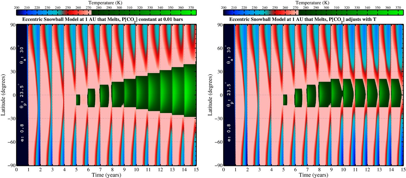
Figure 1 provides a graphical demonstration of the temperature evolution on cold-start planets. Both the left and right panels depict the climate evolution of models with polar obliquity of 23 Figure 1. Temperature evolution maps for cold-start models at 1 AU. Both models have orbital eccentricity of 0.8 along with Earth-like 23 Download figure:5, azimuthal obliquity of 30°, and eccentricity of 0.8. Both models use the WK97 infrared cooling function. In the left panel, the CO2 partial pressure is held constant at 0.01 bars. In the right panel, the CO2 partial pressure begins at 0.01 bars but then, a year after there is positive net melting somewhere on the planet, it adjusts with temperature as described in Section 2.2. For the first ∼9 years, both panels evolve identically. After ∼9 years, an equatorial region of year-round temperate conditions develops. The model in the left panel at this point continues to warm progressively. Once the equatorial region melts, the fraction of surface that has melted ice-cover grows steadily until the entire planet has melted, and temperatures eventually grow to more than 400 K over much of the planet (not shown). In the right panel, in contrast, the thermostat begins to operate after ∼9 years, causing the CO2 concentration to decrease significantly. The negative feedback causes this model to achieve a stable equilibrium climate.
5 polar obliquity and 1 bar surface pressure. Temperature is initialized to 100 K and quickly rises to near 273 K. The melting of the ice-cover is handled in accordance with the prescription of Section 2.2. Left: CO2 partial pressure is held constant at 0.01 bars. In this model, once the equatorial region melts, the region of surface that has melted ice-cover grows steadily until the entire planet has melted, and temperatures eventually grow to more than 400 K over much of the planet (not shown). Right: CO2 partial pressure varies with temperature, in a crude simulation of a "chemical thermostat." In this model, the climate reaches a stable state with equatorial melt regions and polar ice-cover.

We demonstrate in Section 4 that, depending on system architecture, large variations of eccentricity are possible on timescales of less than 106 years. In this context, Table 2 and Figure 1 make it clear that there are possible circumstances in which eccentricity excitation could dramatically warm an initially frozen planet. Intriguingly, in order for a planet to melt out of a snowball state by virtue of increased eccentricity and then to remain with a stable, habitable climate, it might have released some greenhouse gas during its frozen period. In other words, the classical explanation for how the Earth might have exited its own snowball state might need to apply to some extent, although the increased eccentricity can significantly reduce how much greenhouse gas is required.
3.2. Experimenting with a Pseudo-Milankovitch Cycle
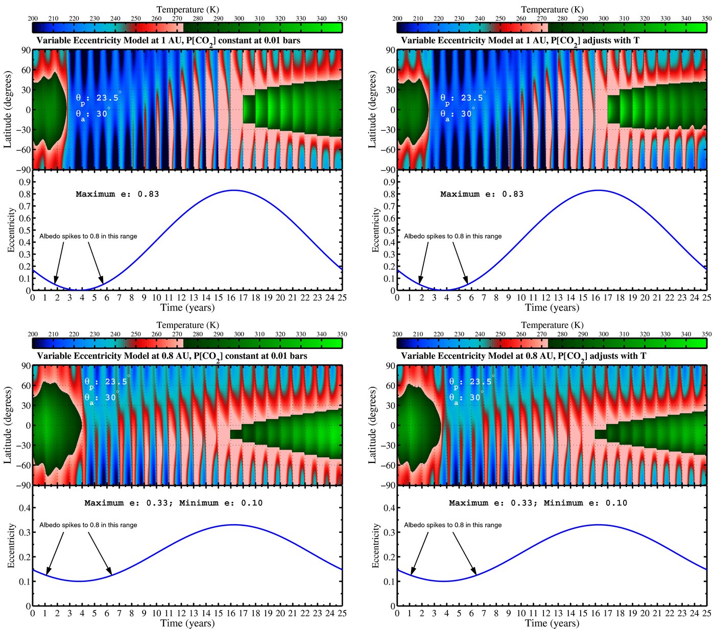
On a real planet with an extreme Milankovitch-like cycle of eccentricity oscillations, the climate never quite reaches a stable year-to-year equilibrium, because the eccentricity is constantly changing. Still, even for the most extreme cases explored in Section 4, the changes in eccentricity are very small from one year to the next, since the periods of eccentricity oscillation are ≳103 years. As a numerical experiment to probe what can happen when eccentricity is varied as a climate model runs, we compress two Milankovitch-like eccentricity cycles into 25 years. One cycle is for a planet at 1 AU, and the other is for a planet at 0.8 AU. For simplicity, we set the eccentricities of both model planets to vary sinusoidally. The 1 AU planet has an extreme Milankovitch-like cycle, with eccentricity varying from 0 to 0.83: e = 0.83{1 + 0.5sin [(t − 10)2π/25]}, and the 0.8 AU planet has a more typical cycle, with eccentricity varying from 0.1 to 0.33. We start both planets with temperate conditions, warm equator, and cold poles (Tinit[λ] = 240 + 60cos2λ). Furthermore, when the eccentricity is below 0.05 for the 1 AU planet and below 0.125 for the 0.8 AU planet, we set the albedo to 0.8, simulating a catastrophic event that plunges the planet into a snowball state in which infrared cooling is governed by IWK97, initially with constant  bars. Figure 2 displays the results of four such model runs (two for planets at 1 AU, two for planets at 0.8 AU; all planets have 235 polar obliquity). In the left panels, the CO2 concentration is held constant at 0.01 bars throughout; in the right panels, the CO2 concentration drops according to the prescription in Section 2.2 once a region of surface has remained above freezing for an entire year. As in Figure 1, the negative feedback of the thermostat's turning on mutes the positive feedback of the ice's melting, resulting in a smaller fraction of the ice-cover melting within the cycle.

Figure 2. Compressed Milankovitch-like evolution of eccentricity and temperature at 1 AU and at 0.8 AU. Planets are initialized with warm equator and cold poles, similar to present-day Earth. In the top row (1 AU), the model planets are the same as in Figure 1, except the eccentricity varies sinusoidally between 0 and 0.83 with a 25 year period, to simulate a time acceleration (by a factor of ∼102 to ∼104) of a Milankovitch-like cycle. When the eccentricity falls below 0.05, the planet's albedo spikes to 0.8, simulating a catastrophic event that plunges the planet into a snowball state, with the latent heat prescription of Section 2.2. In the bottom row (0.8 AU), the eccentricity varies between 0.1 and 0.33, also with a 25 year period. Left: CO2 partial pressure is held fixed at 0.01 bars. As in the left panel of Figure 1, these planets do not establish a temperate equilibrium. Right: CO2 partial pressure varies with temperature. Here, increases in temperature are muted by reduced greenhouse effect once the ice-cover has melted somewhere.
Download figure:
Standard image High-resolution image3.3. Discussion
In Sections 3.1 and 3.2, we presented examples of planets with eccentricities between 0.1 and 0.86, and with eccentricity oscillation cycles of magnitude 0.83 and 0.23. Although oscillations greater than 0.5 in a terrestrial planet's eccentricity (such as those in Figure 2 and some of those in Table 2) might be considered extreme, oscillations of ∼0.3 may be routine. Furthermore, a planet's variable eccentricity need not always return to zero (see the lower right panel of Figure 3), so our galaxy might host many planets whose eccentricities vary between, say, 0.1 and 0.4. Given this, it is worth keeping in mind that the snowball cases considered above might be extreme, as well. Some climate simulations suggest that Earth's snowball state(s) (if in fact it went through any) might have left an equatorial band of open water, perhaps because intense winds (driven by the sharp temperature contrast between frozen and unfrozen tropical ocean) stirred up the typically ∼50 m wind-mixed layer (Hartmann 1994) to much deeper, tapping into the large heat capacity of the deep ocean (Hyde et al. 2000). The idea of a temperate region persisting throughout the (partial) snowball state is also supported by the fact that life evidently survived any such states, which might have been difficult if the whole surface was covered with ice for ≳106 years. Much milder (and more probable) eccentricity excursions could cause a planet in either a partial snowball state or in an analog of Earth's ice ages to warm significantly.

Figure 3. Eccentricity evolution of an Earth-mass planet at 1 AU under the influence of a range of giant planet masses and orbits, labeled by the giant planet (GP) semimajor axes a, eccentricities e, and masses M. Top left: effect of changing the giant planet mass between Saturn's mass and 3 × Jupiter's mass for the case of aGP = 5 AU, eGP = 0.4. Top right: effect of changing the giant planet eccentricity between 0.05 and 0.4 for the case of aGP = 5 AU, MGP = MJup. Bottom left: two cases with similar eccentricity amplitudes but very different planetary system architectures, although both with MGP = MJup: aGP = 0.5 AU, eGP = 0.1 (solid line) and aGP = 5 AU, eGP = 0.4 (dashed line). Bottom right: an extreme case, with aGP = 30 AU, eGP = 0.925, and MGP = 10 MJup (dashed line), and with a = 10 AU, eGP = 0.25, MGP = 10 MJup, and iGP = 75° (solid line).
Download figure:
Standard image High-resolution image
Figure 4. Maximum eccentricity reached by a disk of massless test particles over a million year integration of two systems containing a single Jupiter-mass giant planet in different configurations: aGP = 5 AU, eGP = 0.4 (black dots) and aGP = 0.4 AU, eGP = 0.2 (gray dots).
Download figure:
Standard image High-resolution image
In our models, we have held each planet's obliquity constant (at 235 or 90°, depending on the model). This assumption is purely to limit the complexity of our modeling endeavor; it is not motivated by astrophysical intuition or theory. The architecture of a planetary system affects not only a terrestrial planet's orbital eccentricity, as considered in Section 4, but also its obliquity. Since terrestrial exoplanets' obliquities might vary significantly (Williams 1998a, 1998b), our assumption of constant obliquity restricts the richness of the problem; the evolution of climate and ice-distribution on a planet whose spin-axis direction and orbital eccentricity are both varying wildly is much more complex than we have considered.
Terrestrial exoplanets might someday be discovered that have spectroscopic and photometric characteristics indicative of being covered with snow and ice (and possibly of being shrouded in cold CO2 clouds), i.e., that seem to be in snowball states. If such planets are found, analyzing the full architectures of their planetary systems will allow us to understand whether their eccentricities might vary enough (and on what timescales) to help them melt out of their frozen states. It might even be possible to determine whether a planet is in the process of increasing (or decreasing) its orbital eccentricity, and therefore whether it could be in the process of melting (or freezing), which might, at some point, be testable through direct observations.
4. ORIGIN OF EARTH-LIKE EXOPLANET ECCENTRICITIES
For the purposes of this study, we are interested in the eccentricity evolution of Earth-like planets, in terms of both the amplitude of oscillation and the period of oscillation. Given the importance of resonances and the potential for chaos, it is impossible to understand the detailed dynamical evolution of a planetary system without full knowledge of the system's architecture. However, we can make simple assumptions to get an idea of the range of possibilities. We therefore restrict ourselves to the simple case of an Earth analog at 1 AU evolving under the perturbations from a single massive body, in most cases a Jupiter-mass giant planet. To study these simple, two-planet systems, we numerically integrated the orbits of several systems to look at the range of outcomes and correlations between the perturbing body's mass/orbit and the evolution of the Earth-like planet.
We used two different numerical techniques to integrate our Earth analog—single perturber systems. First, to explore the range of outcomes in coplanar systems, we integrate the orbit-averaged rates of change for the planets' eccentricities e and longitudes of pericenter ϖ using the equations of Mardling & Lin (2002) and Mardling (2007). Our second numerical technique was to directly track the three-dimensional orbits of the planets with the Mercury symplectic integrator (Chambers 1999). We used the orbit-averaged method to study coplanar systems and Mercury to verify the results of the orbit-averaged code and also to study mutually inclined systems. We evolved a variety of systems for 1 Myr, in each case including an Earth-mass planet at 1 AU (initially on a circular orbit) and neglecting the effects of general-relativistic precession. Our simulated systems were chosen not to make predictions about specific known exoplanetary systems but rather to illustrate the variety of eccentricity oscillations of terrestrial planets in dynamically stable (albeit simplified) planetary systems and to show simple correlations between the properties of the perturbing body and the eccentricity of the Earth analog.
The results of our integrations are summarized in Figure 3. The first three panels show the effect of a particular system parameter: the giant planet mass (top left panel), the giant planet eccentricity (top right panel), and the giant planet's orbital distance (bottom right panel). The amplitude of the Earth-like planet's eccentricity oscillation is a function of the giant planet's semimajor axis and eccentricity but is independent of the giant planet's mass (top left panel). However, the oscillation frequency (often referred to as the secular frequency) increases linearly with giant planet mass. The amplitude of the Earth analog's eccentricity oscillation decreases for lower giant planet eccentricities, and the period of oscillation increases with lower giant planet eccentricities (top right panel of Figure 3).
The bottom left panel of Figure 3 shows two systems that both induce eccentricity oscillations of about 0.1 in the Earth analog but on very different timescales of 3000 and 170,000 years. The two systems are markedly different in their architecture: the fast-oscillating case contains a giant planet interior to the Earth-like planet (giant planet at 0.5 AU with an eccentricity of 0.1), and the slow-oscillating case contains an exterior giant planet (at 5 AU with an eccentricity of 0.4).
The first three examples from Figure 3 were chosen such that the giant planets' orbits are consistent with the formation of an Earth-like planet at 1 AU in systems with both inner (Raymond et al. 2006; Mandell et al. 2007) and outer (Raymond 2006) giant planets. For the fourth example, we searched for extreme cases that would be dynamically stable, yet induce very large amplitude oscillations in the Earth analog's eccentricity. One potential source of large eccentricities comes from a consideration of inclinations called the Kozai mechanism (Kozai 1962). For a star–planet-companion system, where the companion can be stellar or planetary, an inclination between the planet and companion's orbits I larger than 392 can induce eccentricity (and inclination) oscillations in the planet's orbit, with a maximum eccentricity emax of
and with a periodicity PKoz of roughly
In Equation 9, M⋆ is the stellar mass, a is semimajor axes, and subscripts 1 and 2 refer to the planet and the companion, respectively (Innanen et al. 1997; Holman et al. 1997; Ford et al. 2000). For reasonable estimates of the mutual inclination between planetary and companion orbits, the majority of binary stars should induce large eccentricity oscillations in any planets that form around the primary star (Takeda & Rasio 2005).
Two extreme cases are shown in the bottom right panel of Figure 3, representing large-scale eccentricity forcing from two dynamical sources: secular forcing in the coplanar system, as seen in the previous examples, and the Kozai mechanism. The secular-forcing example is a system with a 10 Jupiter-mass outer planet at 30 AU with an orbital eccentricity of 0.925.19 In this case, the Earth analog started with an eccentricity of 0.45; thus, the "backstory" for this system involves an impulsive perturbation to the Earth analog that increased its eccentricity considerably, followed by stable secular interactions with the giant planet. The Kozai mechanism example contains a 10 Jupiter-mass planet orbiting at 10 AU with an eccentric and inclined orbit: eccentricity of 0.25 and an inclination of 75° with respect to the Earth-like planet's starting orbital plane. In both cases, the eccentricity of the planet at 1 AU reaches 0.9 or higher on a timescale of one to several hundred thousand years. However, it is important to note that the inclination variations of these planets are markedly different. The system for which the Kozai effect is important induces very large variations in the Earth analog's inclination, going so far as to sometimes rotate in a retrograde sense with respect to its initial orbital plane. In contrast, the secularly forced system remains virtually coplanar.
Resonances and the proximity of the giant planet are both of great importance to the eccentricity evolution of an Earth-like planet. To test these effects, we performed a small number of integrations of systems containing one giant planet and a disk of massless test particles whose behavior represents an ensemble of hypothetical systems with Earth-like planets at different orbital distances. We used the hybrid version of the Mercury integrator, taking care to choose a step size small enough to resolve our innermost orbits at least 20 times. Figure 4 shows the maximum eccentricity reached by test particles in the terrestrial planet zone for two different orbital configurations of a Jupiter-mass planet, one case with the giant planet exterior to 1 AU (shown in black) and one case with the giant planet interior to 1 AU (shown in gray). As expected, the eccentricity decreases farther from the giant planet, in opposite radial directions for the two cases, which induce similar eccentricities in planets at 1 AU. The "blips" in each curve correspond to individual mean motion resonances with the giant planet, which are stronger than in the Solar System because of the giant planets' eccentricities (e.g., Murray & Dermott 2000). The 4:1 resonance with the inner giant planet is visible at 1 AU.
To summarize, the eccentricities of Earth-like planets are determined during either their formation or the subsequent dynamical evolution of the planetary system–in many cases this will include a dynamical instability among the giant planets. Once the system has settled down, the eccentricity of terrestrial planets is determined by the influence of massive perturbers such as giant planets and binary companions, via secular, resonant, and Kozai forcing. For simple systems with a single perturbing planet, the eccentricity oscillation amplitude and period are determined by the giant planet's mass, semimajor axis, and eccentricity. For large mutual inclinations, the Kozai mechanism is governed by the inclination between the planetary and companion orbits and the mass of the companion. The main difference between systems with giant planets interior to the terrestrial planets and systems with giant planets exterior to the terrestrial planets is that the eccentricity oscillation timescale (the secular timescale) is much shorter for close-in giant planet systems. In systems that do not form any giant planets and have no distant companions, there is no obvious mechanism by which large eccentricities should be induced in Earth-like planets. We therefore expect planets in such systems to have relatively circular orbits (Raymond et al. 2007).
The so-called dynamical habitability of planetary systems has been studied via the stability of test particles in the habitable zone of the known extra-solar systems (e.g., Menou & Tabachnik 2003; Barnes & Raymond 2004; Rivera & Haghighipour 2007). This is an interesting exercise because it can help observers by constraining the orbital location of additional planets (see Barnes et al. 2008) and can also test the eccentricity variations of stable test planets. Such stable planets could indeed exist in these systems below the detection threshold and represent Earth analogs.
5. CONCLUSION AND SUMMARY
We have demonstrated that suitably structured exoplanetary systems could contain Earth-like planets that undergo exaggerated versions of Earth's eccentricity Milankovitch cycles. Plausible arrangements of giant and terrestrial planets could lead to an Earth-like planet's eccentricity oscillating between 0 and more than 0.9, on timescales from a few times 103 years to a few times 105 years. Oscillations such as these could have important consequences for climate and habitability.
A companion paper (D10) investigates the influence of a temperate terrestrial planet's eccentricity on its habitability. Here, we have examined that how eccentricity could affect a globally frozen terrestrial planet by introducing an algorithm to allow our EBM to treat the melting of a global ice layer. We found that increasing the eccentricity of an initially frozen model to sufficiently high values can cause the model to melt out of the snowball state. Such high values of eccentricity, however, might place a planet at risk of heating up to temperatures greater than 400 K (perhaps even undergoing a runaway greenhouse effect) if there is not a concomitant negative feedback, such as from a chemical thermostat similar to Earth's carbonate-silicate weathering cycle. Because the climatic influence of increased eccentricity depends on features of a planet's geochemistry that might differ from planet to planet, our results should not be taken as the final word on precisely what values of eccentricity would be required. Nevertheless, the principle remains that if a planet's eccentricity is excited to large values, it is conceivable that there are situations in which this might actually increase, not decrease, its habitability.
The long-term habitability of a planet depends on the properties of its star, on the properties of its own orbit, spin, and geochemistry, and also on the arrangement of other companion planets. When, in the coming years, we find Earth-sized planets at orbital separations that could be consistent with habitable climates, it will be important to study the architectures of those systems, so as to determine what kinds of Milankovitch-like cycles might govern the long-term climatic habitability of such worlds.
We thank Kristen Menou, Frits Paerels, Adam Burrows, Ed Turner, Scott Tremaine, and Brian Jackson for helpful discussions. We thank an anonymous referee for comments and suggestions that materially improved the manuscript. We acknowledge the use of the Della supercomputer at the TIGRESS High Performance Computing and Visualization Center at Princeton University. D.S.S. acknowledges support from NASA grant NNX07AG80G and from JPL/Spitzer agreements 1328092, 1348668, and 1312647. S.N.R. acknowledges funding from NASA Astrobiology Institutes' Virtual Planetary Laboratory lead team, supported by NASA under Cooperative agreement no. NNH05ZDA001C. This research was supported in part by the National Science Foundation under grant no. PHY05-51164.
Footnotes
- 9
- 10
- 11
Even these small variations can cause significant climatic changes (Drysdale et al. 2009).
- 12
Suarez & Held (1979) used a more sophisticated analog of this EBM, but in an Earth-centric context.
- 13
Lorenz (1979) justified the diffusive approximation for studies of large-scale climatic trends; this treatment has been used in many EBMs in the geophysical literature in the last several decades (e.g., Suarez & Held 1979; North et al. 1981, 1983). Furthermore, Showman et al. (2009) provide an illuminating discussion of the applicability of the diffusive approximation. We explored the consequences of varying D in SMS08, SMS09, and D10.
- 14
See Semtner (1976) for a more sophisticated model of the vertical diffusion of heat through an ice layer.
- 15
The estimate of ∼103 years comes from estimating the length of time required to melt a ∼kilometer-thick ice layer at ∼100 cm yr−1, though either the thickness or the rate of melting could differ significantly from these estimates.
- 16
See WK97 for an extensive discussion of the utility and limitations of energy balance climate models in the context of exoplanet climate modeling.
- 17
The work of Le Hir et al. (2009) suggests that it might take significantly longer than we assume for weathering processes to reestablish equilibrium CO2 concentrations after a snowball event.
- 18
Equivalently, it is the angle between the vector from the star to the periastron point and the projection of the planet's spin-vector onto the orbital plane.
- 19