This is the user sandbox of Lms.sworth. A user sandbox is a subpage of the user's user page. It serves as a testing spot and page development space for the user and is not an encyclopedia article. Create or edit your own sandbox here.
Finished writing a draft article? Are you ready to request review of it by an experienced editor for possible inclusion in Wikipedia? Submit your draft for review!
Catastrophic Interference, also known as catastrophic forgetting, is the tendency of a artificial neural network to completely and abruptly forget previously learned information upon learning new information.[1][2]. Neural networks are an important part of the network approach and connectionist approach to cognitive science. These networks use computer simulations to try and model human behaviours, such as memory and learning. Catastrophic interference is an important issue to consider when creating connectionist models of memory. It was originally brought to the attention of the scientific community by research from McCloskey and Cohen (1989)[1], and Ractcliff (1990)[2]. It is a radical manifestation of the ‘sensitivity-stability’ dilemma [3] or the ‘stability-plasticity’ dilemma[4]. Specifically, these problems refer to the issue of being able to make an artificial neural network that is sensitive to, but not disrupted by, new information. Lookup tables and connectionist networks lie on the opposite sides of the stability plasticity spectrum.[5] The former remains completely stable in the presence of new information but lacks the ability to generalize, i.e. infer general priciples, from new inputs. On the other hand, connectionst networks like the standard backpropagation network are very sensitive to new information and can generalize on new inputs. Backpropagation models can be considered good models of human memory insofar as they mirror the human ability to generalize but these networks often exhibit less stability than human memory. Notably, these backpropagation networks are susceptible to catastrophic interference. This is considered an issue when attempting to model human memory because, unlike these networks, humans typically do not show catastrophic forgetting. Thus, the issue of catastrophic interference must be eradicated from these backpropagation models in order to enhance the plausibility as models of human memory.
Artificial Neural Networks: Standard Backpropagation Networks and Their Trainingedit
In order understand the topic of catastrophic interference it is important to understand the components of an artificial neural network and, more specifically, the behaviour of a backpropagation network. The following account of neural networks is summarized from Rethinking Innateness: A Connectionist Perspective on Development by Elman et al (1996). [6]
Figure 1: A three-layer artificial neural network
Artificial neural networks are inspired by biological neural networks. They use mathematical models, namely algorithms, to do things such as classifying data and learning patters in data. Information is represented in these networks through patterns of activation, known as a distributed representations.
The basic components of artificial neural networks are nodes/units and weights.
Nodes or units are simple processing elements, which can be considered artificial neurons. These units can act in a variety of ways. They can act like sensory neurons and collect inputs from the environment, they can act like motor neurons and sent and output, they can act like interneurons and relay information, or they may do all three functions. A backpropagation network is often a three-layer neural network that includes input nodes, hidden nodes, and output nodes (see Figure 1). The hidden nodes allow the network to be transformed into an internal representation, akin to a mental representation. These internal representations give the backpropagation network its ability to capture abstract relationships between different input patterns.
The nodes are also connected to each other, thus they can send activation to one another like neurons. These connections can be unidirectional, creating a feedforward network, or they can be bidirectional, creating a reccurent network. Each of the connections between the nodes has a ``weight``, or strength, and it is in these weights are where the knowledge is ‘stored’. The weights act to multiply the output of a node. They can be excitatory (a positive value) or inhibitory (a negative value). For example, if a node has an output of 1.0 and it is connected to another node with a weight of -0.5 then the second node will receive an input signal of (1.0 x -0.5) = -0.5. Since any one node can receive multiple inputs, the sum of all of these inputs must be taken to calculate the net input.
The net input (neti) to a node j would be defined as:
neti = Σwijoj[2]wij = the weight between node i and joj = the input vector / activation
Once the input has been sent to the hidden layer from the input layer, the hidden node may then send an output to the output layer. The output of any given node depends on the activation of that node and the response function of that node. In the case of a three-layer backpropagation network, the response function is a non-linear, logistic function. This function allows a node to behave in an all or none fashion towards high or low input values and in a more graded and sensitive fashion towards mid-ranged input values. It allows the nodes the result in more substantial changes in the network when the node activation is at the more extreme values. Transforming the net input into a net output that can be sent onto the output layer is calculated by:
oi = 1/[1 +exp(neti)][2]oi = the activation of node i
An important feature of neural networks is that they can learn. Simply put, this means that they can change their outputs when they are given new inputs. Backpropagation, specifically refers to how this the network is trained, i.e. how the network is told to learn. The way in which a backpropagation network learns, is through comparing the actual output to the desired output of the unit. The desired output is known as a 'teacher' and it can be a the same as the input, as in the case of auto-associative/auto-encoder networks, or it can be completely different from the input. Either way, learning which requires a teacher is called supervised learning. The difference between these actual and desired output constitutes an error signal. This error signal is then fedback, or backpropagated, to the nodes in order to modify the weights in the neural network. Backpropagation first modifies the weights between output layer to the hidden layer, then next modifies the weights between the hidden units and the input units. The change in weights help to decrease the discrepancy between the actual and desired output. However, learning is typically incremental in these networks. This means that the these networks will require a series of presentations of the same input before it can come up with the weight changes that will result in the desired output. The weights are usually set to random values for first learning trial and after many trials the weights become more able represent the desired output. The process of converging on an output is called settling. The weights in the This kind of training is based on the error singal and backpropagation learning algorithm / delta rule:
Error signal at output element: e = (ti - oi)oi(1-oi)[2]Error signal at the hidden unit: e = oi(1-oi)Σwike[2]Weight change: Δwij = keoj[2]e= error signal
ti = target output of j
Δwij = the weight change between node i and jwik = new weight calculated from error signal at output element
k = learning rate
o = the activation of node i / actual output of node ioj = the input vector / activation
The issue of catastrophic interference, comes about when learning is sequential. Sequential training involves the network learning an input-output patter until the error is reduced below a specific criterion, then training the network on another set of input-output patterns. Specifically, a backpropagation network will forget information if it first learns input A and then next learns input B. It is not seen when learning is concurrent or interleaved. Interleaved training means the network learns the both inputs-ouput patterns at the same time, i.e. as AB. Weights are only changed when the network is being trained and not when the network is being tested on its response.
To summarize, backpropagation networks:
Involve three-layer neural networks with input, hidden and output units
Use a supervised learning system
Compare the actual output to the target output
Backwards propagate the error signal to update weights across the layers
Learn incrementally through weight updates and eventually settle on the correct ouput
Humans often learn information in a sequential manner. For example, a child will often to learn their 1s addition facts first, later followed by the 2s addition facts, etc. It would be impossible for a child to learn all of the addition facts at the same time. Catastrophic interference can be considered an issue when modelling human memory because, unlike backpropagation networks, humans typically do not show catastrophic forgetting during sequential learning. Rather humans tend to show gradual forgetting or interference when they learn information sequentially. For example, the classic retroactive interference study by Barnes and Underwood (1959)[7] used paired associate learning to determine how much new learning interfered with old learning in humans. Paired associates, means that a pair of stimuli is and responses are learned. Their experiment used eight lists of paired associates, A-B and A-C. The pairs had the stimuli as consonant-vowel-consonant trigrams (e.g, dax) and responses as adjectives. Subjects were initially trained on the A-B list, until they could correctly recall all A-B pairings. Next subjects were given 1, 5, 10 or 20 trials on the A-C list. After learning the A-C pairs the subjects were given a final test in which the stimulus A was presented and the subject was asked to recall the response B and C. They found that as the number of learning trials on A-C list increased, the recall of C increased. But the training on A-C interfered with the recall of B. Specifically recall of B dropped to around 80% after one learning trials of A-C and to 50% after 20 learning trials of A-C. Subsequent research on the topic of retroactive interference has found similar results, with human forgetting being gradual and typically levelling off near 50% recall.[8] Thus when compared with why typical human retroactive interference, catastrophic interference could be likened to retrograde amnesia. [1]
Some researchers have argued that catastrophic interference is not an issue with the backpropagation model of human memory. For example, Mirman and Spivey (2001) found that humans show more interference when learning pattern-based information[9]. Pattern-based learning is analogous to how a standard backpropagation network learns. Thus, they concluded that catastrophic interference is not limited to connectionist memory models but rather that it is a "general product of patterm-based learning that occurs in humans as well" (p.272).[9] However, Musca, Rousset and Ans (2004) found contrasting results where retroactive interference was more pronounced in subjects who sequentially learned unstructured lists when controlling for methodological failure that occurred in the Mirman, D., & Spivey, M. (2001) study. [10]
The term catastrophic interference was originally coined by McCloskey and Cohen (1989) but was also brought to the attention of the scientific community by research from Ractcliff (1990)[2].
The Sequential Learning Problem: McCloskey and Cohen (1989)edit
McCloskey and Cohen(1989) noted the problem of catastrophic interference during two different experiments with backpropagation neural network modelling.
Experiment 1: Learning the ones and twos addition facts
In their first experiment they trained a standard backpropagation neural network on a single training set consisting of 17 single-digit ones problems (i.e, 1 +1 through 9 + 1, and 1 + 2 through 1 + 9) until the network could represent and respond properly to all of them. The error between the actual output and the desired output steadily declined across training sessions, which reflected that the network learned to represent the target outputs better across trials. Next they trained the network on a single training set consisting of 17 single-digit twos problems (i.e, 2+1 through 2 + 9, and 1 + 2 through 9 + 2) until the network could represent, respond properly to all of them. They noted that their procedure was similar to how a child would learn their addition facts. Following each learning trial on the twos facts, the network was tested for its knowledge on both the ones and twos addition facts. Like the ones facts, the twos facts were readily learned by the network. However, McCloskey and Cohen noted the network was no longer able to properly answer the ones addition problems even after one learning trial of the twos addition problems. The output pattern produced in response to the ones facts often resembled an output pattern for an incorrect number more closely than the output pattern for an incorrect number. This is considered to be a drastic amount of error. Furthermore, the problems 2+1 and 2+1, which were included in both training sets, even showed dramatic disruption during the first learning trials of the twos facts.
Experiment 2: Replication of Barnes and Underwood (1959) study[7]
In their second connectionist model, McCloskey and Cohen attempted to replicate the study on retroactive interference in humans by Barnes and Underwood (1959). They trained the model on A-B and A-C lists and used a context pattern in the input vector (input pattern), to differential between the lists. Specifically the network was trained to responds with the right B response when shown the A stimulus and A-B context patter and to respond with the correct C response when shown the A stimulus and the A-C context pattern. When the model was trained concurrently on the A-B and A-C items then network readily learned all of the associations correctly. In sequential training the A-B list was trained first, followed by the A-C list. After each presentation of the A-C list, performance was measured for both the A-B and A-C lists. They found that, the amount of training on the A-C list in Barnes and Underwood study that lead to 50% correct responses lead to nearly 0% correct responses by the backpropagation network. Furthermore, they found that the network tended to show responses that looked like the C response pattern when the network was prompted to give the B response pattern. This indicated that the A-C list apparently had overwritten the A-B list. This could be likened to learning the word dog, followed learning the word stool and then finding that you cannot recognize the word cat well but instead think of the word stool when presented with the word dog.
McCloskey and Cohen tried to reduce interference through a number of manipulations including changing the number of hidden units, changing the value of the learning rate parameter, overtraining on the A-B list, freezing certain connection weights, changing target values 0 and 1 instead 0.1 and 0.9. However none of these manipulations satisfactorily reduced the catastrophic interference exhibited by the networks.
Overall, McCloskey and Cohen (1989) concluded that:
at least some interference will occur whenever new learning alters the weights involved representing
the greater the amount of new learning, the greater the disruption in old knowledge
interference was catastrophic in the backpropagation networks when learning was sequential but not concurrent
Constraints Imposed by Learning and Forgetting Functions: Ratcliff (1990)edit
Ratcliff (1990) used multiple sets of backpropagation models applied to standard recognition memory procedures, in which the items were sequentially learned.[2] After inspecting the recognition performance models he found two major problems:
Well-learned information was catastrophically forgotten as new information was learned in both small and large backpropagation networks.
Even one learning trial with new information resulted in significant of the old information, paralleling the findings of findings of McCloskey and Cohen (1989).[1] Ratcliff also found that the resulting outputs were often a blend of the previous input and the new input. In larger networks, items learned in groups (e.g. AB then CD) were more resistant to forgetting than were items learned singly (e.g. A then B then C…). However, the forgetting for items learned in groups was still large. Adding new hidden units to the network did not reduce interference.
Discrimination between the studied items and previously unseen items decreases at the network learned more.
This finding contradicts with studies on human memory, which indicated that discrimination increases with learning. Ratcliff attempted to alleviate this problem by adding ‘response nodes’ that would selectively respond to old and new inputs. However, this method did not work as these response nodes would become active for all inputs. A model which used a context pattern also failed to increase discrimination between new and old items.
Many researchers have suggested that the main cause of catastrophic interference is overlap in the representations at the hidden layer of distributed neural networks. [11][12][13] In a distributed representation any given input will tend to create changes in the weights to many of the nodes. Catastrophic forgetting occurs because when many of the weights, where ‘knowledge is stored, are changed it is impossible for prior knowledge to be kept intact. During sequential learning, the inputs become mixed with the new input being superimposed over top of the old input.[12]. Another way to conceptualize this is through visualizing learning as movement through a weight space.[14] This weight space can be likened to a spatial representation of all of the possible combinations of weights that the network can possess. When a network first learns to represent a set of patterns, it has found a point in weight space which allows it to recognize all of the patterns that is has seen.[13] However, when the network learns a new set of patterns sequentially it will move to a place in the weight space that allows it to only recognize the new pattern.[13] To recognize both sets of patterns, the network must find a place in weight space that can represent both the new and the old output. One way to do this is by connecting a hidden unit to only a subset of the input units. This reduces the likelihood that two different inputs will be encoded by the same hidden units and weights and so will decrease the chance of interference.[12] Indeed, a number of the proposed solutions to catastrophic interference involve reducing the amount of overlap that occurs when storing information in these weights.
Many of the early techniques in reducing representational overlap involved making either the input vectors or the hidden unit activation patterns orthogonal to one another. Lewandowsky and Li (1995) [15] noted that the interference between sequentially learned patterns is minimized if the input vectors are orthogonal to each other. Input vectors are said to be orthogonal to each other if the pairwise product of their elements across the two vectors sum to zero. For example the patterns [0,0,1,0] and [0,1,0,0] are said to be orthogonal because (0x0 + 0x1 + 1x0 + 0x0) = 0. One of the techniques which can create orthogonal representations at the hidden layers involves bipolar feature coding (i.e., coding using -1 and 1 rather than 0 and 1)[13]. Orthogonal patterns tend to produce less interference with each other. However not all learning problems can be represented using these types of vectors and some studies report that the degree of interference is still problematic with orthogonal vectors.[2] Simple techniques such varying the learning rate parameters in the backpropagation equation were not successful in reducing interferece. Varying the number of hidden nodes has also been used to try and reduce interference. However, the findings have been mixed with some studies finding that more hidden units decrease interference [16] and other studies finding it does not.[1][2]
Below are a number of techniques which have empirical support in successfully in reducing catastrophic interference in backpropagation neural networks:
French(1991) [11] proposed that catastrophic interference arises in feedforward backpropagation networks due to the interaction of node activations, or activation overlap, that occur in distributed representations at the hidden layer. Specifically, he defined this activation overlap as the average shared activation over all units in the hidden layer, calculated by summing the lowest activation of the nodes at the hidden layer and averaging this sum. For example, if the activations at the hidden layer from one input are (0.3, 0.1, 0.9, 1.0) and the activations from the next input are (0.0, 0.9, 0.1, 0.9) the activation overlap would be (0.3 + 0.1 + 0.1 + 0.9 )/ 4 = 0.35. When using [binary number|binary] representation of input [row vector|vectors], activation values will be 0 through 1, where 0 indicates no activation overlap and 1 indicates full activation overlap. French noted that neural networks which employ very localized representations do not show catastrophic interference because the lack of overlap at the hidden layer. That is to say, each input pattern will create a hidden layer representation that involves the activation of only one node, so differed inputs will have an activation overlap of 0. Thus, he suggested that reducing the value of activation overlap at the hidden layer would reduce catastrophic interference in distributed networks. Specifically he proposed that this could be done through changing the distributed representations at the hidden layer to ‘semi-distributed’ representations. A ‘semi-distributed’ representation have fewer hidden nodes that are active, and/or a lower activation value for these nodes, for each representation, which will make the representations of the different inputs overlap less at the hidden layer. French recommended that this could be done through ‘activation sharpening’, a technique which slightly increases the activation of a certain number of the most active nodes in the hidden layer, slightly reduces the activation of all the other units and then changes the input-to-hidden layer weights to reflect these activation changes (similar to error backpropgation). Overall the guidelines for the process of ‘activation sharpening’ are as follows:
Perform a forward activation pass by feeding an input from the input layer to the hidden layer and record the activations at the hidden layer
“Sharpen” the activation of x number of most active nodes by a sharpening factor α:
       Anew = Aold + α(1- Aold) 		For nodes to be sharpened, i.e. more activated
       Anew = Aold – αAold	           For all other nodes
French suggested the number of nodes to be sharpened should be log n nodes, where n is the number of hidden layer nodes
Use the difference between the old activation (Aold) and the sharpened activation (Anew) as an error, backpropagate this error to the input layer, and modify the weights of input-to-output appropriately
Do a full forward pass with the input through to the output layer
Backpropagate as usual from the output to the input layer
Repeat
In his tests of an 8-8-8 (input-hidden-output) node backpropagation network where one node was sharpened, French found that this sharpening paradigm did result in one node being much more active than the other seven. Moreover, when sharpened, this network took one fourth the time to relearn the initial inputs than a standard backpropagation without node sharpening. Relearning is a measure of memory savings and thus extent of forgetting, where more time to relearn suggests more forgetting (Ebbinghaus savings method). A two-node sharpened network performed even slightly better, however if more than two nodes were sharpened forgetting increased again.
According to French, the sharpened activations interfere less with weights in the network than unsharpened weights and this is due specifically to the way that backpropagation algorithm calculates weight changes. Activations near 0 will change the weights of links less than activations near 1. Consequently, when there are many nodes with low activations (due to sharpening), the weights to and from these nodes will be modified much less than the weights on very active,nodes. As a result when a new input is fed into the network, sharpening will reduce activation overlap by limiting the number of highly active hidden units and will reduce the likelihood of representational overlap by reducing the number of weights that are to be changed. Thus, node sharpening will decrease the amount of disruption in the old weights, which store prior input patterns, thereby reducing the likelihood of catastrophic forgetting.
Kortge (1990) [17] proposed a learning rule for training neural networks, called the ‘novelty rule’, to help alleviate catastrophic interference. As its name suggests, this rule helps the neural network to learn only the components of a new input that differ from an old input. Consequently, the novelty rule changes only the weights that were not previously dedicated to storing information, thereby reducing the overlap in representations at the hidden units. Thus, even when inputs are somewhat similar to another, dissimilar representations can be made at the hidden layer. In order to apply the novelty rule, during learning the input pattern is replaced by a novelty vector that represents the components that differ. The novelty vector for the first layer (input units to hidden units) is determined by taking the target pattern away from the current output of the network (the delta rule). For the second layer (hidden units to output units) the novelty vector is simply the activation of the hidden units that resulted from using the novelty vector as an input through the first layer. Weight changes in the network are computed by using a modified delta rule with the novelty vector replacing the activation value (sum of the inputs):
Δwij = kδidi
Δwij = weight change between nodes i and jk = learning rate,
δi = error signel
di= novely vector
When the novelty rule is used in a standard backpropagation network there is no, or lessened, forgetting of old items when new items are presented sequentially [17]. However, this rule can only apply to auto-encoder or auto-associative networks, in which the target response for the output layer is identical to the input pattern. This is because the novelty vector would be meaningless if the desired output was not identical to the input as it would be impossible to calculate how much a new input differed from the old input.
McRae and Hetherington (1993)[12] argued that humans, unlike most neural networks, do not take on new learning tasks with a random set of weights. Rather, people tend to bring a wealth of prior knowledge to a task and this helps to avoid the problem of interference. They proposed that when a network is pre-trained on a random sample of data prior to starting a sequential learning task that this prior knowledge will naturally constrain how the new information can be incorporated. This would occur because a random sample of data from a domain which has a high degree of internal structure, such as the English language, training would capture the regularities, or recurring patterns, found within that domain. Since the domain is based off of regularities, a newly learned item will tend to be similar to the previously learned information, which will allow the network to incorporate new data with little interference with existing data. Specifically, an input vector which follows the same pattern of regularities as the previously trained data should not cause a drastically different pattern of activation at the hidden layer or a drastically alter weights.
To test their hypothesis, McRae and Hetherington (1993) compared the performance of a naïve and pretrained auto-encoder backpropagation network on three simulations of verbal learning tasks. The pre-trained network was trained using letter based representations of English monosyllabic words or English word pairs. All three tasks involved the learning of some consonant-vowel-consonant (CVC) strings or CVC pairs (list A), followed by training on a second list of these items (list B). Afterwards, the distributions of the hidden node activations were compared between the naïve and pre-trained network. In all three tasks, the representations of a CVC in the naïve network tended to be spread fairly evenly across all hidden nodes, whereas most hidden nodes were inactive in the pre-trained network. Furthermore, in the pre-trained network the representational overlap between CVCs was reduced compared to the naïve network. The pre-trained network also retained some similarity information as the representational overlap between similar CVCs, like JEP and ZEP, was greater than for dissimilar CVCs, such as JEP and YUG. This suggests that the pre-trained network had a better ability to generalize, i.e. notice the patterns, than the naïve network. Most importantly, this reduction in hidden unit activation and representational overlap resulted in significantly less forgetting in the pre-trained network than the naïve network, essentially eliminating catastrophic interference. Essentially, the pre-training acted to create internal orthogonalization of the activations at the hidden layer, which reduced interference. [13] Thus, pre-training is a simple way to reduce catastrophic forgetting in standard backpropagation networks.
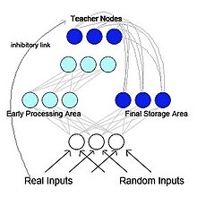
French (1997) proposed the idea of a pseudo-reccurent backprobabgation network in order to help reduce catastrophic interference (see Figure 2). [5] In this model the network is separated into two functionally distinct but interacting sub-networks. This model is biologically inspired and is based on research from McClelland, McNaughton, and O’Reilly (1995). [18]. In this research McClelland et al. (1995), suggested that the hippocampus and neocortex act as separable but complementary memory systems. Specifically, the hippocampus short term memory storage and acts gradually over time to transfer memories into the neocortex for long term memory storage. They suggest that the information that is stored can be “brought back” to the hippocampus during active rehearsal, reminiscence, and sleep and renewed activation is what acts to transfer the information to the neocortex over time. In the pseudo-recurrent network, one of the sub-networks acts as an early processing area, akin to the hippocampus, and functions to learn new input patters. The other sub-network acts as a final-storage area, akin to the neocortex. However, unlike in McClelland et al. (1995) model, the final-storage area sends internally generated representation back to the early processing area. This creates a recurrent network. French proposed that this interleaving of old representations with new representations is the only way to reduce radical forgetting. Since the brain would most likely not have access to the original input patterns, the patterns that would be fed back to the neocortex would be are internally generated representations called pseudopatterns. These pseudopatterns approximations of previous inputs [19] and they are can be interleaved with the learning of new inputs. Figure 2: The architecture of a pseudo-recurrent networkThe use of these pseudopattern could be biologically plausible as parallels between the consolidation of learning that occurs during sleep and the use of interleaved pseudopatterns. Specifically, they both serve to integrate new information with old information without disruption of the old information. [20] When given an input (and a teacher value) is fed into the pseudo-recurrent network would act as follows:
When a pattern is fed from the environment (a real input), the information travels both to the early processing area and the final storage area, however the teacher nodes will inhibit the output from the final storage area
The new pattern is learned by the early processing area by the standard backpropagation algorithm
At the same time random input is also fed into the network and causes pseudopatterns to be generated by the final storage area
Output from the final-storage area, in the form of pseudopatterns, will be used as a teacher for the early-processing area. In this way, the pseudopatterns are interleaved with the ‘real inputs’ from the environment
Once the new pattern and the pseudopattern are learned by the early processing area, its weights are copied to the corresponding weights in the final storage area.
When tested on sequential learning of real world patterns, categorization of edible and poisonous mushrooms, the pseudo-recurrent network was showed less interference than a standard backpropagation network. This improvement was with both memory savings and exact recognition of old patterns. When the activation patterns of the the pseudo-recurrent network were investigated, it was shown that this network automatically formed semi-distributed representations. Since these types of representations involve fewer nodes being activated for each pattern, it is likely what helped to reduce interference.
Not only did the pseudo-recurrent model show reduced interference but also it models list-length and list-strength effects seen in humans. The list-length effect means that adding new items to a list harms the memory of earlier items. Like humans, the pseudo recurrent network showed a more gradual forgetting when to be trained list is lengthened. The list-strength effect means that when the strength of recognition for one item is increased, there is no effect on the recognition of the other list items. This is an important finding as other models often exhibit a decrease in the recognition of other list items when one list item is strengthened. Since the direct copying of weights from the early processing area to the final storage area does not seem highly biologically plausible, the transfer of information to the final storage area can be done through training the final storage area with psuedopatterns created by the early processing area. However, a disadvantage of the pseudo-recurrent model is that the number of hidden units in the early processing and final storage sub-networks must be identical.
Prominent Researchers in Catastrophic Interferenceedit
^ abcdeMcCloskey, M. & Cohen, N. (1989) Catastrophic interference in connectionist networks: The sequential learning problem. In G. H. Bower (ed.) The Psychology of Learning and Motivation,24, 109-164
^ abcdefghijkRatcliff, R. (1990) Connectionist models of recognition memory: Constraints imposed by learning and forgetting functions. Psychological Review,97, 285-308
^Hebb, D.O. (1949). ``Organization of Behaviour``. New York: Wiley
^Caroebterm G., & Grossberg, S. (1987) ART 2: Self-organization of stable category recognition codes for analog input patterns. ``Applied Optics, 26``, 4919-4930
^ abFrench, R. M. (1997) Pseudo-recurrent connectionist networks: an approach to the ‘sensitivity-stability’ dilemma. Connection Science, 9(4), 353–379.
^ Elman, J., Karmiloff-Smith, A., Bates, E., & Johnson, M. (1996). ``Rethinking Innateness: A Connectionist Perspective on Development.`` Cambridge, MA: MIT Press.
^ abBarnes, J. M., & Underwood, B. J. (1959). Fate of first-list associations in transfer theory. Journal of Experimental Psychology, 58, 97–105.
^Postman, L., & Underwood, B. J. (1973). Critical issues in interference theory. Memory & Cognition, 1(1), 19-40.
^ abMirman, D., & Spivey, M. (2001). Retroactive interference in neural networks and in humans: the effect of pattern-based learning. Connection Science, 13(3), 257-275
^ Musca, S.C., Rousset, S & Ans, B. (2004). Differential retroactive interference in humans following exposure to structured or unstructured learning material: a single distributed neural network account. Connection Science, 16(2), 101-118
^ ab French, R. M. (1991). Using Semi-Distributed Representations to Overcome Catastrophic Forgetting in Connectioniost Networks. In: Proceedings of the 13th Annual Cognitive Science Society Conference (pp. 173-178) New Jersey: Lawrence Erlbaum.
^ abcd McRae, K., & Hetherington, P. (1993). Catastrophic Interference is Eliminated in Pre-Trained Networks. In: Proceedings of the 15th Annual Conference of the Cognitive Science Society (pp. 723-728). Hillsdale, NJ: Lawrence Erlbaum
^ abcdeFrench, R. M. (1999). Catastrophic forgetting in connectionist networks. Trends in Cognitive Sciences, 3(4), 128–135.
^Lewandowsky S. (1991). Gradual unlearning and catastrophic interference: a comparison of distributed architectures. In: Hockley WE and Lewandowsky S (eds). Relating theory and data: essays on human memory in honor of Bennet B. Murdock (pp. 445–476). Hillsdale, NJ: Lawrence Erlbaum
^Lewandowsky, S., & Li, S-C. (1995). Catastrophic interference in neural networks: causes, solutions, and data. In: Dempster, F.N. & Brainerd, C. (eds). Interference and Inhibition in Cognition (pp. 329–361). San Diego: Academic Press
^Yamaguchi, M. (2004). Reassessment of Catastrophic Interference. Computational Neuroscience, 15(15), 2423 - 2426
^ ab Kortge, C. A. (1990). Episodic memory in connectionist networks. In: The Twelfth Annual Conference of the Cognitive Science Society, (pp. 764-771). Hillsdale, NJ: Lawrence Erlbaum.
^McClelland, J., McNaughton, B. & O'Reilly, R. (1995) Why there are complementary learning systems in the hippocampus and neocortex: Insights from the successes and failures of connectionist models of learning and memory. Psychological Review, 102, 419-457.
^Robins, A. (1995). Catastrophic Forgetting, rehearsal and pseudorehearal. Connection Science, 7, 123-146.
^Robins, A. (1996). Consolidation in Neural Networks and in the Sleeping Brain. Connection Science, 8(2), 259-276.